CS 76 / 176

Why probabilistic reasoning?

• Imperfect measurement of data. (hidden state)
• Imperfect computation (e.g. chess)
• Randomized algorithms?

Review of probability

Random variables: variable that take on values based on some distribution.

Example: $\{x\}$, a boolean-valued random variable.
We write $x$ to denote $\{x\} = \mathrm{true}$.

$P(a)$: probability that $\{a\} = \mathrm{t}$

$P(\neg a)$: probability that $\{a\} = \mathrm{f}$

Independent variables

Independent variables:

$P(a \wedge b) = P(a) P(b)$

but $P(a \vee b)$ is not $P(a) + P(b)$.

Flip a coin twice. Let $P(h_1)$ be probability of heads first flip. Let $P(h_2)$ be probability of heads second flip.

$P(h_1 \vee h_2) \ne 1$

Use DeMorgan to compute $P(a \vee b)$:

$P(a \vee b) = P(\neg(\neg a \wedge \neg b))$

$P(a \vee b) = 1 - P(\neg a \wedge \neg b)$

Independent variables

From DeMorgan:

$P(a \vee b) = 1 - P(\neg a \wedge \neg b)$

If $\{a\}, \{b\}$ are independent:

$P(a \vee b) = 1 - P(\neg a) P(\neg b)$

$P(a \vee b) = 1 - (1 - P(a)) (1 - P(b))$

or, $P(a) + P(b) - P(a \wedge b)$

$P(a \vee b)$ is colored area in the figure. In the figure, if you add $P(a) + P(b)$, then $P(a \wedge b)$ is double-counted.

Joint distributions

$\neg a \wedge \neg b$

$a \wedge \neg b$

$\neg a \wedge b$

$ a \wedge b$

Joint distributions

$\neg a \wedge \neg b$

$a \wedge \neg b$

$\neg a \wedge b$

$ a \wedge b$

Joint distributions

Assume we have $3$ random variables $\{x\}$, $\{y\}$, $\{z\}$.

There are $2^3$ possible outcomes: $(0, 0, 0)\ldots (1, 1, 1)$.

Red cube is the outcome $x \enspace \neg y \enspace z$, or $(1 \enspace 0 \enspace 1)$.

Joint distributions

The joint distribution gives all information needed to compute any probability.

$P(x) =$

$P(x \enspace \neg y \enspace \neg z)$ +

$P(x \enspace \neg y \enspace z)$ +

$P(x \enspace y \enspace \neg z)$ +

$P(x \enspace y \enspace z)$

Joint distributions

The joint distribution gives all information needed to compute any probability.

$P(x \vee y) = P(x) + P(y) - P(x \enspace y)$ (double counting)

Marginalizing over $z$,

$= P(x) + P(y) - ( P(x \enspace y \enspace \neg z) + P(x \enspace y \enspace z)) = $

$P(x \enspace \neg y \enspace \neg z) + P(x \enspace \neg y \enspace z) + P(x \enspace y \enspace \neg z) + P(x \enspace y \enspace z) +$

$ P(\neg x \enspace y \enspace \neg z) + P(\neg x \enspace y \enspace z) + P(x \enspace y \enspace \neg z) + P(x \enspace y \enspace z) -$

$P(x \enspace y \enspace \neg z) - P(x \enspace y \enspace z)$

Joint distributions

If we stored $2^n$ values of the joint distribution, we would be able to compute any probability we wanted.

Problems with joint probabilities:

• Computational cost exponential in number of vars.
• Data starvation: how likely is each outcome? Each outcome must appear many times for measurement of joint probabilities.

Conditional probabilities

(Dependence between variables.)

$P(a | b)$ is the probability that $\{a\} = \mathrm{t}$,
given that we know that $\{b\} = \mathrm{t}$.

Chaining of probabilities:

$P(a \wedge b) = P(a) P(b | a)$

What's the chance of a dart landing in $a$? Ok, now that it has, what percentage of $a$ is covered by $b$?

Symmetrically,

$P(a \wedge b) = P(b) P(a | b)$.

Conditionals from joint distribution

$P(a \wedge b) = P(a) P(b|a)$ (chaining)

$P(b|a) = \frac{P(a \wedge b)}{P(a)}$ (division)

$P(b|a) = \frac{P(a \enspace b)}{P(a \enspace \neg b) + P(a \enspace b)}$ (marginalize over $b$)

Causality, independence

$P(b|a) = P(b)$ iff $a$ and $b$ are independent.

$a$: aliens land

$b$: building on fire

Bogus claim: $b$ is dependent on $a$, but $a$ is not dependent on $b$.

Bogus reasoning: causally, $a \rightarrow b$.

1. Alien landings cause buildings to alight (heat guns).
2. But we can't just light a bunch of buildings on fire and wait for the aliens. (Some people try this.)

Causality, independence

(In)dependence is two-way, regardless of the causal relationship.

In other words, knowing that a building is on fire tells us that there may be aliens nearby, and knowing that the aliens have landed is good reason to tell the fire trucks to be ready.

Bayes rule

How are conditional probabilities $P(a|b)$ and $P(b|a)$ related?

$P(a | b) = \frac{P(a) P (b|a)}{P(b)}$,

which is not hard to derive:

$P(a \wedge b) = P(a \wedge b)$

$P(a) P(b| a) = P(b) P(a | b)$

Bayes rule is useful when we know a sensor model. For example, maybe we know the probability of the sensor triggering if there isi really a wall. But we want to know the probability of a wall, given that the sensor triggered.

Review of probability

• Random variables: variables that take on values based on some distribution. $\{x\}$
• Joint probability: likelihood of a complete model/ assignment. $P(x \wedge \neg y \wedge z)$.
• Marginalizing: $P(x)$ = $P(x \wedge y) + P(X \wedge \neg y)$.
• Conditional probability: Probability of some variable value, given that we know the values of some other variables already. (Restricted model space.)
• Chaining: $P(a \wedge b) = P(a | b) P(b)$
• Bayes rule: $P(a | b) = P(a) P(b | a) / P(b)$
• Independence: $P(a | b) = P(a)$. Also $P(a \wedge b) = P(a)P(b)$.

Bayesian networks

Joint distributions have some problems:

• Marginalizing is expensive.
• Large memory requirements for joint distribution.
• Limited number of experiments implies data starvation.

But what if the problem has some structure, based on independence of variables?

Conditional independence

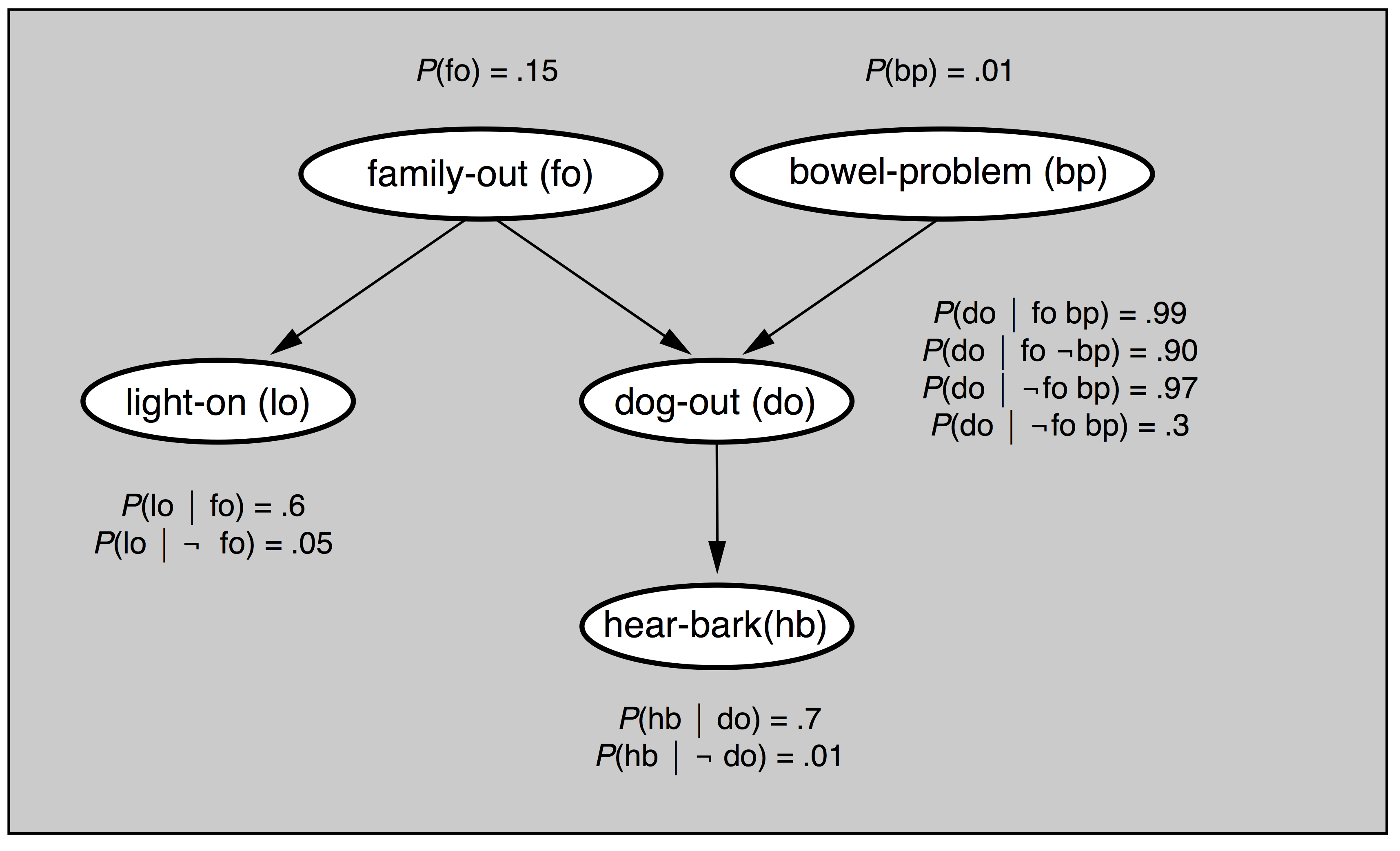
Assume I hear a bark and notice that the light is on. What is $P(bp)$? We could use the $2^{32}$ joint probabilities.

But notice that if the dog is known to be out, then hear-bark is independent of bowel-problem or family-out:

$P(hb | do \wedge bp) = P(hb | do) = .7$

$P(hb | do \wedge fo) = P(hb | do) = .7$

Probabilistic reasoning over time

(A special case of a graphical model.)

Each time slice contains a snapshot of a set of variables, some observable, some not.

State variables $X_1 \ldots X_n$ are not observable.

Evidence variables $E_1 \ldots E_n$ are observable.

$X_i$ and $E_i$ are themselves vectors of variables.

Markov models

1. Cause precedes effect:
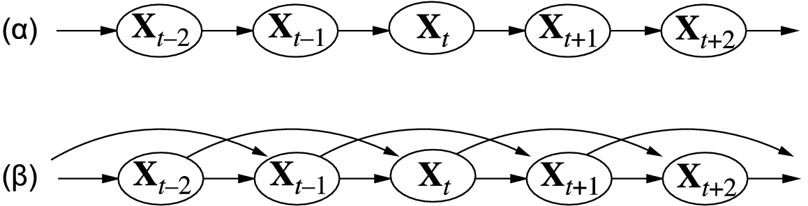
2. Markov assumption: the probability of a state depends on a finite history of previous states.

The figure shows first-order and second-order Markov processes.

Markov assumption

Assume $b_i$ is drink beer on day $i$.

If I drink a beer today, it is more likely that I will drink a beer tomorrow. Our model might have the property:

$P(b_2 | b_1) > P(b_2) > P(b_2 | \neg b_1)$

and further,

$P(b_3 | b_1, b_2) > P(b_3| b_2) > P(b_3 | b_1)$

$> P(b_3) > P(b_3| \neg b_1)$

$> P(b_3 | \neg b_2) > P(b_3 | \neg b_1, \neg b_2)$

Markov assumption

Or assume that we are trying to predict the next word that will be said. (Or was said, but garbled.)

You heard: "Four-score and seven ... rglbrarf"

$P(\mathrm{years} | \mathrm{fourscore, and, seven}) >>$ $P(\mathrm{years} | \mathrm{seven})$

$P(\mathrm{years} | \mathrm{seven}) > P(\mathrm{years})$

The dependence could be arbitrarily long-distance. Maybe the next word I'm going to say is "Lincoln".

Markov assumption

Maybe probabilities depend on prior knowledg ein a very complex way. In what year was the Gettysburg address?

"Four-score and seven years ago" is in reference to the date of the Declaration of Independence:

$1776$ + $87$ = $1863$

But taking long-distance dependencies into account is a hard A.I. problem; Turing's original challenge.

So we make a Markov assumption: the probability of a state depends on a finite history of previous states.

Conditional independence

Second-order Markov Process (MP):

$P(X_{10}| X_{0:9})$ = $P(X_{10} | X_8, X_9)$

First-order Markov Process:

$P(X_{t}| X_{0:t - 1})$ = $P(X_{t} | X_{t - 1})$

Still, sometimes bad. If I say "Hurricane strikes Florida, the news at 6," the probability of hearing "hurricane" at 6:05 pm is elevated.

First-order models

Any higher-order Markov model can be expressed as a 1st-order Markov model. $X_8, X_9$ can be viewed as a single vector-valued variable.

It is equivalent to say

1. "today's stock price depends only on the past two daily stock prices" or
2. "(the stock prices for today and yesterday) depends only on the stock prices for (yesterday and the day before)".

Define new variables $Y_{10} = (X_9, X_{10})$ and $Y_{9} = (X_9, X_8)$

Hidden Markov models

Each time slice contains a snapshot of a set of variables, some observable, some not.

State variables $X_1 \ldots X_n$ are not observable.

Evidence variables $E_1 \ldots E_n$ are observable.

Evidence

We assume that the evidence variables $E$ depend only on the current state:

$P(E_t | X_{0:t}, E_{0:t - 1})$ = $P(E_t | X_t)$

We might call this the sensor model: the thermomenter reading depends only on the current temperature.

But it's only conditional independence. If you don't know the current temperature...

Assumption bogus when:

1. Sensor itself has state. (Cold temp. broke thermom.)
2. Something else is unmodeled.

Umbrella world

Notice that we have enough information to compute the entire joint distribution if we want to. (No data starvation, but expensive.)

HMM Joint distribution

$P(X_0, X_1, X_2, \ldots X_t, E_1, E_2, \ldots E_t) = P(X_{0:t} E_{1:t})$

Split out $X_0$:

$= P(X_0)$ $ P(X_{1:t} E_{1:t}| X_0)$

Split out $E_t$:

$=P(X_0)$ $P(E_t | X_{0:t} E_{1:t-1})$ $P(X_{1:t} E_{1:t-1} | X_0)$

(Notice that $|X_0$ is carried along behind.)

HMM Joint distribution

$P(X_0, X_1, X_2, \ldots X_t, E_1, E_2, \ldots E_t)$

$=P(X_0)$ $P(E_t | X_{0:t} E_{1:t-1})$ $P(X_{1:t} E_{1:t-1} | X_0)$

Conditional independence:

$=P(X_0)$ $P(E_t | X_t)$ $P(X_{1:t} E_{1:t - 1}| X_0)$

We're making progress. Red part involves fewer variables than where we began. Now split out $X_t$:

HMM Joint distribution

$P(X_0, X_1, X_2, \ldots X_t, E_1, E_2, \ldots E_t)=$

Conditional independence:

$P(X_0)$ $P(E_t | X_t)$ $P(X_t | X_{t- 1})$ $P(X_{1:t - 1} E_{1:t - 1} | X_0)$

Now we're really getting somewhere. The red stuff is very similar to what we had before we started, but with $X_t$ or $E_t$ deleted! (And with a carried $X_0$.)

$= P(X_0) \prod_i^t P(X_i | X_{x-1}) P(E_i|X_i)$

HMM Joint distribution

$P(X_0, X_1, X_2, \ldots X_t, E_1, E_2, \ldots E_t)=$

$= P(X_0) \prod_i^t P(X_i | X_{x-1}) P(E_i|X_i)$

So, you can compute any joint probability in linear time given only the sensor model and the state update model:

Temporal inference

Four questions (Dickens three ghosts):

1. Filtering/ monitoring (present): What is the belief state (the posterior distribution over current state) given a stream of evidnce starting at $t=1$?

   Compute $P(X_t | e_{1:t})$

2. Prediction (future): Compute posterior distribution over the future, given evidence to date:

   Compute $P(X_{t + k} | e_{1:t}$ for some $k > 0)$

(Note: capitals indicate true/false distr, lowercase, t/f.)

Temporal inference

3. Smoothing/ hindsight (past): Given all evidence up to present, compute posterior distribution for a past state.

   Compute $P(X_k | e_{1:t})$, for $k < t$.

4. Most likely explanation: given a sequence of evidence, compute a most-likely sequence of states (speech recognition, etc):

   Compute ${\operatorname{argmax}}_{X_1:t} P(X_{1:t} | e_{1:t})$

Filtering and prediction

Recursive formulation: there exists some function $f$:

$P(X_{t+1} | e_{1: t + 1}) = f(e_{t + 1}, P(X_t | e_{1:t}))$

Filter will have two parts: predict then update.

$X_{t}$

$X_{t + 1}$

$e_{t + 1}$

predict

update

Filter: derivation

Compute $P(X_{t+1} | e_{1:t+1})$

1. Divide the evidence (just notational):

   $ = P(X_{t+1}| e_{t + 1}, e_{1:t})$

2. Bayes rule: swap $X_{t + 1}$ and $e_{t + 1}$, carrying along $|e_{1:t})$:

   $ = P(e_{t + 1} | X_{t + 1}, e_{1:t}) \cdot \frac{P(X_{t + 1}|e_{1:t})}{P(e_{t + 1}| e_{1:t})}$

Filter: derivation

From last step, $P(e_{t + 1} | X_{t + 1}, e_{1:t}) \cdot \frac{P(X_{t + 1}|e_{1:t})}{P(e_{t + 1}| e_{1:t})}$

3. Normalize. What is ${P(e_{t + 1}| e_{1:t})}$? No idea. But $P(X_{t+1})$, distribution including both true and false. Sum of probabilities for true and false must be 1. So let $\alpha$ be a normalizing constant:

$ = \alpha P(e_{t + 1} | X_{t + 1}, e_{1:t}) \cdot P(X_{t + 1}|e_{1:t})$

4. Markov property of evidence:

$ = \alpha $ $P(e_{t + 1} | X_{t + 1})$ $P(X_{t + 1} | e_{1:t})$

Filter: derivation

We have:

$\alpha $ $P(e_{t + 1} | X_{t + 1})$ $P(X_{t + 1} | e_{1:t})$.

$\alpha$ update prediction

To do the prediction, we will condition on current state $X_t$. (Either $X_t$ is true, or it is false.)

Filter: derivation

Computing prediction $P(X_{t + 1} | e_{1:t})$. by conditioning on current state $X_t$:

$\sum_{x_t} P(X_{t+1}| x_t, e_{1:t}) P(x_t|e_{1:t})$

By Markov property,

$\sum_{x_t}$ $P(X_{t+1}| x_t)$ $P(x_t|e_{1:t})$

Transition model State distribution

Filtering

$X_{t}$

$X_{t + 1}$

$e_{t + 1}$

predict

update

new state estimate =

$\alpha $ $P(e_{t + 1} | X_{t + 1})$ $\sum_{x_t} P(X_{t+1}| x_t)$ $P(x_t|e_{1:t})$

$\alpha$ update transition prev. state estimate

Filtering example

Assuming we saw the umbrella on days 1 and 2, what is the posterior distribution over the state? (Is it raining on day 2?)

Day 0, probability of rain is .5 (prior $P(R_0) = \langle .5, .5 \rangle$)

Day 1: prediction

Prediction from $t = 0$ to $t = 1$ is:

$P(R_1) = \sum_{r_0 \in \{t, f\} } P(R_1| r_0) P(r_0)$

$P(R_1) = \langle .7, .3 \rangle \times .5 + \langle .3, .7 \rangle \times .5 = \langle .5, .5 \rangle$

Day 1: update

Update with evidence for $t = 1$ (saw umbrella):

$P(R_1 | u_1) = \alpha P(u_1 | R_1) P (R_1)$

$ = \alpha \langle .9 . 2 \rangle \langle .5 .5 \rangle$ (element by element mult.)

$ = \alpha \langle .45, .1 \rangle $ $ = \langle .818, .182 \rangle $

Day 2: prediction

Prediction from $t = 0$ to $t = 1$ is:

$P(R_2 | u_1) = \sum_{r_1 } P(R_2| r_1) P(r_1|u_1)$

$ = \langle .7, .3 \rangle \times .818 + \langle .3, .7 \rangle \times .182$

$ = \langle .627, .373 \rangle $

Day 2: update

$P(R_2 | u_1, u_2) = \alpha P(u_2 | R_2) P(R_2 | u_1)$

$= \alpha \langle .9, .2 \rangle \langle .627, .373 \rangle$

$= \alpha \langle .565, .075 \rangle$ $= \langle .883, .117 \rangle$

Filtering: review

1. Prior distribution: choose a distribution $X_0$ that gives probability of each state initially. (A vector of probabilities associated with the values in order. What if there are multiple variables?)
2. Prediction step: Each state (value) has a probability vector that gives probability of transitioning to every new possible state. For each state in current distribution, take probability of being in that state, multiply by associated vector, and add up the results.

Filtering: review

3. Sensor update step: Given the current evidence (sensor reading), choose the vector describing sensor probabilities of that evidence for each possible state. Do element-by-element multiplication to get a new estimate of the state.
4. Normalize: But the sensor update was wrong, because we really should have used probability of state given sensor reading, obviously. Bayes rule says that we're only off by a constant factor, though, and since it's the same constant for all states, we can just normalize.

Prediction

We already know how to do it. Just keep predicting, skip the update step.

Stationary distribution: prediction limit as $k \rightarrow \infty$

For the rain example,

$\lim_{k \rightarrow \infty} P(X_{t + k}| e_{1:t}) = \langle .5, .5 \rangle$

Mixing time: time to get "close" to stationary distribution

Smoothing sequences

What if we wanted to smooth a whole sequence?

Could do forwards to each state, then backwards: $O(n^2)$ time, $O(n)$ memory to store results.

Faster, a forwards-backwards algorithm:

1. Run all the way forwards, storing result at each step (the forward messages)
2. Run all the way backwards, storing backwards messages
3. Combine messages

Forwards-backwards

Used for speech recognition, text smoothing, data smoothing.

Drawbacks:

1. Not online (consider fixed-lag smoothing)
2. Not a way to find most-likely sequence

Most-likely sequence

Bad idea: compute posteriors using smoothing, and choose most-likely state at each step.

Problem: posteriors are over single time step.

Example: Consider speech recognition with the microphone broken. Lots of possible sentences, and in most of them, the character e is likely at any given position.

So, was the most-likely sequence eeeeeeeee?

Viterbi algorithm

Viterbi algorithm. Each sequence is a path through the graph whose nodes are possible states.

Subsequences of optimal paths are optimal!

Viterbi algorithm

Take example where we reach $R_5 = true$. The path is either

1. optimal to $R_4 = true, R_5 = true$ or
2. optimal to $R_4 = false, R_5 = true$

So, find optimal paths to both possible states for $R_4$, and then test which of them is better to $R_5 = true$.

Viterbi algorithm

There's a formula in the book (15.11), but just a BFS, with state transitions based on max probabilities:

Used for most-likely sequence of words, amino acids, robot or world states...

Log tricks

Every sequence is unlikely, if long enough.

But we are only choosing the maximum, and $\log(x) > \log (y)$ (monotonic increasing). And $\log(a \cdot b \cdot c) = \log(a) + \log(b) + \log(c)$...

Matrix formulation

1. The distribution over state is a vector of probabilities.
2. The prediction step is a linear sum of transition probability vectors, weighted by probability of being in each state.
3. The update step is just element-by-element multiplication of current distribution with sensor model.

Matrix-vector multiplication

A simple rule for combining some numbers:

$\mathbf{Ax} = \begin{pmatrix} a & b & c \\ p & q & r \\ u & v & w \end{pmatrix} \begin{pmatrix} x_1 \\ x_2 \\ x_3 \end{pmatrix} =\begin{pmatrix} ax_1 + bx_2 + cx_3 \\ px_1 + qx_2 + rx_3 \\ ux_1 + vx_2 + wx_3 \end{pmatrix} $

But also, a weighted sum of columns: $\mathbf{Ax} = x_1 \begin{pmatrix} a \\ p \\ u \end{pmatrix} + x_2 \begin{pmatrix} b \\ q \\ v \end{pmatrix} + x_3 \begin{pmatrix} c \\ r \\ w \end{pmatrix}$

Prediction matrix

Prediction step: Each state (value) has a probability vector that gives probability of transitioning to every new possible state. For each state in current distribution, take probability of being in that state, multiply by associated vector, and add up the results.

So, if we take the transition probabilities for each state, and stack them into a column, multiplying this matrix by the current distribution gives the predicted distribution.

Prediction matrix

Example:

$T^T = P(X_t | X_{t - 1}) = \begin{pmatrix} .7 & .3 \\ .3 & .7 \end{pmatrix}$

(First column is transition probabilities for 'raining=false'. Standard state transition matrix has row per state.)

$P(R_1) = \begin{pmatrix} .7 & .3 \\ .3 & .7 \end{pmatrix} \begin{pmatrix} .5 \\ .5 \end{pmatrix}$

$ = .5 \begin{pmatrix} .7 \\ .3 \end{pmatrix} + .5 \begin{pmatrix} .3 \\ .7 \end{pmatrix}$ $ = \begin{pmatrix} .5 \\ .5 \end{pmatrix} $

Observation matrix

Element-by-element multiplication of two vectors: take one vector and make it into a diagonal matrix. In this case, create an observation matrix:

$O_{u} = \begin{pmatrix} .9 & 0 \\ 0 & .2 \end{pmatrix}$

$O_{\neg u} = \begin{pmatrix} .1 & 0 \\ 0 & .8 \end{pmatrix}$

Select the matrix based on the current evidence.

Example 1

$P(R_2 | u_1, u_2) = \alpha O_u T^T O_u T^T \begin{pmatrix} .5 \\ .5 \end{pmatrix}$

$ = \begin{pmatrix} .883 \\ .117 \end{pmatrix}$

Notes:

1. Normalize once.
2. Transition same, but observation matrix changes.
3. Multiply right-to-left, because matrix-vector mult is faster than matrix-matrix.

Example 2

$P(R_2 | u_1, u_2, \neg u_3, \neg u_4, u_5)$

$= \alpha O_u T^T O_{\neg u} T^T O_{\neg u} T^T O_u T^T O_u T^T \begin{pmatrix} .5 \\ .5 \end{pmatrix}$

Note order: $t = 0$ is on the right.

Stationary distributions

No evidence $\Rightarrow$ no observation matrices to select:

$P(R_5 | \emptyset) = T^T T^T T^T T^T T^T \begin{pmatrix} .5 \\ .5 \end{pmatrix}$

Or, if we let $A = T^T$ and $\mathbf{x_i} = P(X_i)$:

$\mathbf{x_n} = A^n \mathbf{x_0}$

Given some prior $x_0$, we expect the distribution of states to 'settle out' at some eventual stationary distribution.

Pagerank

1. Consider the internet as a graph; pages are vertices
2. Humans start uniformly distributed over vertices
3. Let them do a random walk, by selecting a random link

In the limit, what is the distribution of people over pages?

$\mathbf{x_n} = A^n \mathbf{x_0}$

We just need to compute $A^n$ as $n \rightarrow \infty $. How big is $A$?

Problems: $A$ is $m \times m$, computationally expensive. Also, some pages have no links leaving, and some pages are not reachable by links.

Pagerank

1. To solve the 'no links' problem, allow some random teleporting. (Small probability of randomly moving somewhere else.)
2. Use sparse matrix storage method.
3. $x_n$ is an eigenvector of $A^n$.

Eigenvectors of a matrix are vectors that are only scaled when multiplied by that matrix. Not all matrices have real eigenvectors (consider rotation matrix), but expect certain matrices to (ergodic Markov chains, possible to go from every state to every other state, eventually).

Pagerank

Cayley-Hamilton theorem allows one to compute any power of $A^n$ without computing any power higher than $m$, the rank of the matrix.

Pagerank uses sparse-matrix tricks based on the Cayley-Hamilton theorem to compute eigenvectors of $A^n$ fairly quickly, using an iterative procedure.