Robot modelling: kinematics
What is a robot? Robotics researchers are interested in the interaction of physical systems and computers. There are controlled mechanical systems, like microwaves, cars, or dishwashers, that we do not tend to think of as robots. There are also traditional robotics applications where the robot follows fixed trajectories, and has little interaction with the environment. We should keep open minds about what constitutes an interesting problem in robotics.
Robot of the day: brachiating 2R arm (Nishimura and Funaka).
Robots as technology
Robots scale human abilities. Robots can precisely manipulate small objects, forcefully manipulate large objects, move quickly, repeatably, or at a distance. Example applications include
- Factory automation
- Field robotics
- Service and entertainment
- Medical and scientific devices
The most widespread application of robotics has been industrial automation. Some of the challenges include removing uncertainty in part orientation, repeatable motion, avoiding jamming due to friction during assembly, and designing the product for ease of assembly or disassembly.
The ability to move precisely and operate hygienically at a distance has motivated the use of robots for scientific experiments and medicine.
Robots are also used for space exploration, hazardous waste cleanup, and to deliver medicine in hospitals. There are current projects to build autonomous cars, and personal assistants for the elderly or disabled.
Robots as science
Programmable mechanisms also allow exploration of fundamental scientific questions. What information is needed about the environment to complete a manipulation task, and how should that information be represented or stored? How do biological systems manage complicated manipulation so effectively? What can we learn about social interaction from our reactions to robotic mechanisms? Robots allow hands-on (well, grippers-on) experiments that are very suitable for education.
- Mechanics of manipulation and locomotion
- Biologically-inspired robots
- Education
Robot programming paradigms
A useful abstraction for robot programming divides systems into two parts: the robot, and the world. The robot is the part of the system that we can control. The goal is to change the world. The robot receives information about the state of the world through sensors, plans an action based on the history of sensor readings, (current belief about the state of the world), and executes the action.

This paradigm drives the high-level design of much robot control software: the main loop senses the state, makes a plan, and then sends commands to the motors.
Throughout much of the course, we will focus on planning and action. However, the interaction between action and sensing can be interesting. For example, sometimes action can reduce the effects of sensor error. Consider dropping a marble into a funnel. We might not know the exact initial position of the the marble; there is much less uncertainty about the marble’s position after it has fallen through the funnel.
Mechanisms: joints and linkages
Joints constrain the motion between pairs of rigid bodies. For example, a revolute joint constrains the relative motion between the bodies to pure rotation. A linear prismatic joint only allows linear translation along an axis. There are some stylized symbols used to draw diagrams of linkages, collections of joints and rigid bodies (or links).

These symbols also allow some simple 3D mechanisms to be drawn in flat configurations without the need for a complicated perspective drawing.

The classification of linkages as parallel, branching, or serial in the figure depends on whether the arrangement of links and joints forms loops (also called cycles) or not. We will see later that computing the possible motions of parallel mechanisms can be difficult.
We use some notation to loosely describe the type of a serial robot arm. For example, an RR arm would indicate a serial arm with two revolute joints. A PR arm would indicate an arm with a prismatic joint and a revolute joint, in that order starting from the ground. We shorten this even further if there are multiple joints of the same type in a row – a 2R arm has two revolute joints.
The two serial mechanisms in the figure above are a 2R and an RP arm.
We also talked about the relationship between symmetry and joints, and looked at other possible types of joints, including ball joints, screw joints, and plane-plane joints.
Linkages as devices for computation
Linkages provide the transmission between the motors and the world in robots, but they can do more than that. For example, consider the problem of computing the value of \(\sin(x)\). One approach would be to write a computer program that computes an an approximation using a series expansion. Another approach would be to build a linkage composed of an arm of length one connected by a revolute joint to another arm, like this:

The “input” for this computational machine is the joint angle, and the “output” is the length of the perpendicular from the arm of length one to the other arm. We have a name for this mechanism – it’s a protractor! Slide rules are another example of a clever way to compute a function mechanically. I wonder what class of functions can be approximated arbitarily well by a planar mechanism composed of only rigid links, and revolute and prismatic joints?
The reason this idea is more than a curiosity is that clever linkage design can be one way of “programming” robot motion. A beautiful example of this is passive dynamic walking.
Degrees of freedom
The configuration of a linkage can be described using a few numbers. Let’s look at a few examples. A triangular rigid body in the plane can be described using three numbers. For example, you could use \(x\) and \(y\) coordinates to describe the location of one of the corners of the triangle. You could then use a coordinate \(\theta\) to describe the angle that one of the edges makes with some coordinate system. We say that the triangle in the plane has three degrees of freedom.
There is a 2R serial arm in one of the figures above. It is rigidly attached to the ground, and has two revolute joints. We could use two numbers to describe the configuration of the arm: \(\theta_1\) and \(\theta_2\), the angles through which each joint has rotated from some initial configuration. The serial 2R arm has two degrees of freedom.
Exercise: counting degrees of freedom
Consider your arm, including your shoulder, and imagining your hand as a rigid paddle that you can move, but not bend; we will ignore fingers. How many degrees of freedom does your arm have? Why?
Reuleaux collection of mechansims
There is a brilliant collection of different types of mechanisms that was built by Reuleaux in the 19th century. Cornell now has this collection and has a web page describing each mechanism:
Reuleaux mechanisms at Cornell
Workspaces for branching and serial mechanisms (graphical method)
Think about a robot arm bolted to the ground. The distal point on the arm is called the end effector, and is a natural place to put a tool of some type – fingers, a screw driver, or an arc welder. The set of points that the end effector can reach is called the robot workspace. Given a mechanism, what is its workspace? Here’s an example with a planar 2R arm.
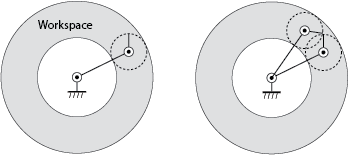
First, imagine all joints fixed (locked in place) except the last one. In our case, that means fixing the first joint. Move the last joint through its full range. In the general case, there might be limits on the range of motion of the joint, but in this case, the last joint can move freely; the end effector moves along the dashed circle shown in the left figure. This is the workspace of the last joint, assuming the other joints are fixed.
Now free the next joint closer to the ground, and move that joint through its full range of motion, dragging the workspace we’ve already constructed. In this case, the first joint drags the dashed circle in a big circle. The region that is swept out is a “donut”, or annulus; this is the workspace for the arm.
Not all points in the workspace are the same. The figure on the right shows that there are two ways (or configurations of the arm) in which the end effector can reach any point on the interior of the workspace. We call these two configurations elbow up and elbow down configurations of the arm.
Each point on the outer boundary of the workspace can only be reached in one way (with the second joint fully extended, and the first joint at a particular angle), and each point on the inner boundary of the workspace can only be reached one way – with the second joint fully flexed.
This difference between the boundary of the workspace and the interior is interesting and important. Notice that for arm configurations in the interior, it is possible to move the effector instantaneously in any direction. However, for a point on the boundary, it is not possible to achieve an instantaneous velocity for the end effector that points inwards – first you have to bend the second joint, then you can move the effector inwards or outwards. We’ll look at this phenomenon (called singularities of mechanisms) more closely when we study differential kinematics, but you might already be familiar with some uses of it: stiff-arming someone, standing straight to lift a heavy weight, or holding a suitcase with your arm at full extension.
Exercise: Drawing workspaces with joint limits
Consider a 2R planar arm with. Let the first link have length 2, and be constrained to move in the range \([-\pi/4, \pi/4]\). Let the first link have length 1, and be constrained to move in the range \([0, \pi/2]\). Draw the reachable workspace for the end effector.
Forward kinematics of 2R planar arms
Consider a simple planar 2R arm. The configuration is given by \((\theta_1, \theta_2) \in S \times S\).

What is the location of the end effector? The location of the first joint is:
\(\left( \begin{array}{c} x_1 \\ y_1 \end{array} \right) = \left( \begin{array}{c} l_1 \cos \theta_1 \\ l_1 \sin \theta_1 \end{array} \right)\)
The location of the end effector is
\(\left( \begin{array}{c} x \\ y \end{array} \right) = \left( \begin{array}{c} l_1 \cos \theta_1 + l_2 \cos (\theta_1 + \theta_2) \\ l_1 \sin \theta_1 + l_2 \sin(\theta_1 + \theta_2) \end{array} \right)\)
It’s annoying to write long terms like \(\sin(\theta_1 + \theta_2)\), and what if we
have five links?
We use a notational shorthand for sine
\(s_{1 2... n} = \sin(\theta_1 + \theta_2 + ... + \theta_n)\)
and have a similar notation for cosine.
With this notation, the location of the effector is:
\(\left( \begin{array}{c} x \\ y \end{array} \right) = \left( \begin{array}{c} l_1 c_1 + l_2 c_{12} \\ l_1 s_1 + l_2 c_{12} \end{array} \right)\)
In general, we write the forward kinematics in the form
\(\left( \begin{array}{c} x_1 \\ x_2 \\ \vdots \\ x_n \end{array} \right) = f(q)\)
\(f(q)\) is a vector-valued function of a vector: it takes \(d\) arguments (where \(d\) is the dimension of the configuration space), and gives \(n\) values (where \(n\) is the dimension of the point whose location we would like to know.)
Sometimes, a forward kinematics map might give information other than just the locations of points. Let’s say we want to know the angle of the end effector, as well as its position. (The angle is probably important, since you can’t pick something up with the back of your hand!) Write \(q_e = (x_e, y_e, \theta_e)\) to be the configuration of the end-effector system. (The end-effector system is a subset of the robot system!)
\(q_e = \left( \begin{array}{c} l_1 c_1 + l_2 c_{12} \\ l_1 s_1 + l_2 s_{12} \\ \theta_1 + \theta_2 \end{array} \right)\)
Inverse kinematics for planar arms
Forward kinematics tells us where a point on a robot arm is, assuming we know the angles at all the joints. This can be useful (especially for checking for things like collisions), but what we probably really want to know is what joint angles to set to reach some given point in space. The mapping from locations in the workspace to points in configuration space is called the “inverse kinematics” of the arm.
For serial manipulators, the inverse kinematics problem is typically much more challenging than the forward kinematics problem. Given a chain of homogeneous transform matrices, and the location of the point, we need to solve for the \(\theta\) values, and they are inside the sines and cosines.
Even for our simple 2R planar arm example, solving for \(\theta_1\) and \(\theta_2\) is going to take a little work:
\(\left( \begin{array}{c} x \\ y \end{array} \right) = \left( \begin{array}{c} l_1 \cos \theta_1 + l_2 \cos (\theta_1 + \theta_2) \\ l_1 \sin \theta_1 + l_2 \sin(\theta_1 + \theta_2) \end{array} \right)\)
Inverse kinematics for planar 2R arm, geometric approach
The trick is to draw a right triangle inscribing the arm as shown. Then compute the length of the hypotenuse for that triangle: \(c^2 = x^2 + y^2\). Now we can use the law of cosines to compute the angle capital \(C\), by looking at the triangle formed by the hypotenuse and the two links of the arm. We have
\(c^2 = l_1^2 + l_2^2 - 2 l_1 l_2 \cos C\)
Solve for C using an inverse cosine, making sure to get the correct solution for the inverse cosine by inspection. Then \(\theta_2 = \pi - C\). (Notice that there is an alternate solution for \(\theta_2\) as well. I’ll leave it as an exercise how to get that alternate solution.)
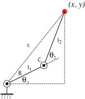
Now notice that we can solve for the angle B using the law of sines on the same triangle. Once we have \(B\), notice that \(\theta_1 + B = \tan^{-1}(y, x)\), the two-argument arctangent of the initial point.
Solving transcendental equations by reduction to polynomial
How would you solve the inverse kinematics of a more complicated arm using the law of cosines approach? I would not want to. You could also take an algebraic approach and attempt to directly solve the kinematic equations, and for the 2R arm, such a solution requires only a fair amount of cleverness.
However, there is a nice systematic way to solve problems of this sort. The difficulty with solving transcendental equations is that for each variable \(\theta_i\), both a sine and a cosine term may appear. There’s also some issue with the summations inside the sines and cosines.
The summation issue is solved easily for planar arms: measure the angles from the horizontal, rather than with respect to the previous frame – at the end, we can just subtract to get the actual joint angles.
The sines and cosines can be eliminated by observing that if we let \(u = \tan(\theta/2)\), then
\(\cos \theta = \frac{1 - u^2}{1 + u^2}\)
and
\(\sin \theta = \frac{2u}{1 + u^2}.\)
This is sometimes called the Weierstrass substitution.
Craig’s Introduction to Robotics text gives the example of solving the equation
\(a \cos \theta + b \sin \theta = c.\)
Making the substitution and multiplying through by \(1 + u^2\), we get
\(a ( 1 - u^2) + 2bu = c(1 + u^2)\)
which after collecting powers of u is
\((a + c) u^2 - 2 b u + (c - a) =0.\)
Solve for \(u\) with the quadratic formula, and take the inverse tangent to solve for \(\theta/2\).
Inverse kinematics for more complicated arms
Inverse kinematics of complicated arms may need to be solved numerically, since general closed-form solutions are not known to find the roots of polynomials of greater than degree 4. However, certain special cases are known. For example, six-DOF arms are common, since six degrees of freedom allows full control over the pose of a rigid body in space. Work by Pieper solves the inverse kinematics in the special case where three of the joint axes intersect at a point, and in fact, this has influenced the design of real robot arms.
Parallel manipulators
In some sense, the forward kinematics for a serial manipulator are “easy”, and the inverse kinematics are “hard”. For a parallel manipulator, we expect the opposite to be true. We can think of a parallel manipulator as being made up of a collection of simple serial manipulators, joined in some way (either by a built-in joint, or by a joint formed when each serial manipulator grabs the same object).
Here’s a nice video of a linkage that draws a straight line: