Configuration space

For a 2R planar arm, setting values for \(\theta_1\) and \(\theta_2\) determines the complete configuration of the arm: where every molecule of the arm is located. There is a space of configurations for the arm that corresponds to the range of possible \(\theta_1\) and \(\theta_2\) values for the arm. We will discuss the idea of configuration space more formally later in the course.

Obstacles

A point in the configuration space corresponds to a particular configuration of the system. If there are obstacles, some configurations of the system will not be possible. We call the space of configurations that do not collide with obstacles the free configuration space; we call the space of points in configuration space that cause collisions the “configuration space obstacles”. Every continuous trajectory that lies within the free configuration space corresponds to a motion of the robot that will not cause a collision; writing algorithms to find such trajectories is a central problem in the robotics literature.

Visualizing configuration spaces

Paramaterizations sometimes allow us to visualize configuration spaces. For example, consider a 2R planar arm with no joint limits. We might use the angles \(\theta_1\) and \(\theta_2\) to represent configurations. We could then graph \(\theta_1\) vs \(\theta_2\). Each point on the graph represents a unique configuration of the arm. A path would represent a connected set of configurations that can be reached by continuous motions of the joints. Notice that the graph “wraps around” – a path that goes off the graph at \(2\pi\) wraps to zero, and should be considered connected. (Remember that the topology of the configuration space for a 2R arm is actually a torus – we can visualize this by thinking of the graph on a piece of paper, rolling the paper into a tube to glue the top and bottom edges of the paper together, and then curving the tube into a donut to glue the left and right edges of the paper together.)

Some points in the configuration space will correspond to cases where the arm collides with an obstacle. The set of points in the configuration space that do not collide with any obstacle is called the free configuration space. The set of points that do cause collisions are called the configuration space obstacles.

Planning a collision free motion for the robot (which might be very complicated – imagine a snake robot, for example!) then can be abstractly formulated as the problem of planning a path for a point robot among obstacles in the configuration space.

It is very convenient to always be able to think about motion planning problems as planning paths for a point, but there is a problem: finding the locations of the configuration-space obstacles is usually hard. There are a few special cases that we will examine: 2R planar arms, and rigid bodies in the plane.

Obstacles for 2R planar arms

Here is a 2R planar arm, with one point obstacle in the physical space:

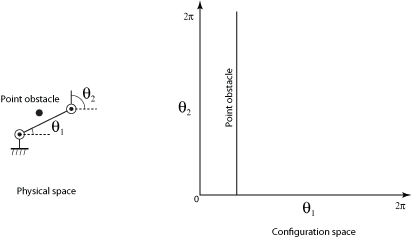
The location of the obstacle is such that only the first link can collide with it, and that link collides at about \(\theta_1= \pi/4\). Since the collision happens for every value of \(\theta_2\), the configuration space obstacle looks like a line in the graph of the configuration space the right.

What would happen if the placement of the obstacle was such that link 2 could collide with it? The situation would be much more complicated. The cspace obstacle is the set of configurations where there is a collision, so you could imagine sliding link 2 along the obstacle, while causing link 1 to comply with that motion.

Planar translation of rigid bodies

Here is a triangular planar robot that can only translate, and some polygonal obstacles:

We will describe the configuration of the robot by the location of a reference point attached to the robot. The configuration space is therefore \(\mathbf R^2\). As we drag the robot around by its reference point, there will be intersections between the robot and the obstacles. We mark those \((x, y)\) configurations as collisions in the configuration space, as shown in pink below.

There’s a pattern to the set of points where there are collisions, and we can use this pattern to derive a graphical method for constructing the configuration space obstacles. Imagine an obstacle that is just a point. For what configurations of the robot does that particular point collide with the robot? Slide the robot edges around the point, marking the location of the reference point as you slide. You’ll find that you get a shape in configuration space that looks like a flipped version of the robot – a reflection of the robot in \(x\) and \(y\) across horizontal and vertical lines through the reference point.

Notice that the boundaries of the polygonal obstacles are unions of point obstacles. The configuration space obstacles are therefore unions of flipped robots. So, to construct the configuration space obstacles, flip the robot, drag it around the boundary of all the physical obstacles, and that will give you the shapes of the configuration space obstacles.

It’s not surprising that the c-space obstacles are larger than the original physical obstacles – the robot has ‘shrunk’ to a point.

Translations and rotations of rigid bodies in the plane

What if the rigid body can rotate as well as translate? We might describe the configurations using the location of the reference point, together with an angle describing how far the robot has rotated from some base configuration. We parameterize the configuration space by three numbers: \((x, y, \theta)\). We can graph \(\theta\) on the z axis, so long as we remember that it wraps from 0 to \(2\pi\).

Obstacles will then be volumes in the configuration space. It’s harder to visualize the boundaries of cspace obstacles, but we can use the trick from the previous section to visualize slices of obstacles. Choose \(\theta = 0\). This is a robot that can only translate, and we can draw this slice of the cspace by flipping the robot and dragging around the boundaries of obstacles. Now choose some other value of \(\theta\). The robot has rotated, but as long as we maintain that value of \(\theta\), the rotated robot only translates. So flip the rotated robot, and drag along the boundaries.

If we choose all values of \(\theta\) (or more practically, choose some discrete sampling), we can construct the cspace obstacles in slices.

You can imagine that it is possible to analytically construct the boundaries of obstacles for planar rigid bodies. This is correct, but harder than you might think. See Randy Brosts’s Ph.D. thesis, or more recent work by Elisha Sacks, for details.

Other abstract spaces

The state of a system is the set of quantities that we are interested in. For physical systems, we are often interested in the location of all the particles, so the state of the system is its configuration. A configuration space is therefore a special case of a state space.

In other disciplines, we might be interested in other quantities, but the idea of thinking about associating a point in a space with each state in the system is common. For example, in physics, it is typical to be interested in the motion of particles or rigid bodies together with their momenta, since Hamiltonian formulation of the dynamics equations are expressed in terms of momenta. The phase space of a system is the set of configurations of the particles and their momenta. That is, the phase space is the Cartesian product of the configuration space with the momentum space.

In control theory or the study of systems of differential equations, we are interested in both variables and derivatives of those variables. If those variables describe a phsyical system, they might describe a configuration of the system. Derivatives would then correspond to velocities of the physical system. A point in the state space of the dynamic system assigns a value to each variable and its derivative.

In computer science, the states of a system are often discrete. The discrete state space of the system can therefore be represented by a graph showing the connectivity of the different states. Consider a chess board, for example. An AI to play chess would consider the state of a single piece to be its location on the board, and the state of the entire game to be the location of every piece on the board. Each individual chess piece is analogous to a particle, and the set of chess pieces is analogous to a system of particles.