Discretizing continuous spaces
Graph-search algorithms like breadth-first search, depth-first search, iterative deepening, uniform-cost search, greedy best-first search, A, and variants can find a path between two nodes in a graph. Given a clean, discrete graph, these algorithms have nice properties. For example, A makes good use of a heuristic to reduce running time, while still optimizing path cost; iterative deepening can be used to find optimal paths while reducing memory requirements. What do we do if the space is continuous? If you only have a hammer, everything looks like a nail. So one choice is to discretize the problem, and then search. The discretization (we hope) will capture some essential characteristics of the problem. Then the path can be refined to make sure that it is smoother and actually reaches the goal.
There are many ways to discretize a search problem. Let’s start with a simple example, planning a path for a point robot among polygonal obstacles. Assume we would like to find the shortest path between start and goal. We could cut the world up into little grid cells, mark each cell as “occupied” or “not occupied” depending on whether an obstacle overlaps the cell, and do some sort of (A*, IDS, BFS…) search on the space.
A few questions come up:
- How big should the cells be?
- How close to an optimal answer will we get?
- How expensive is this algorithm? What about in 3d? State space grows exponentially with dim. (The curse of dimensionality.)
- Is this algorithm complete? (No, it’s “resolution complete”.)
We will make certain assumptions. We will assume that the robot can move freely in any direction in configuration space (if there is not an obstacle there), that the obstacles don’t move (or if they do, they move along fixed paths), that the environment is known fully ahead of time, and that the configuration space obstacles can be constructed.
For almost all motion planning problems we will make use of key abstraction: the configuration of the robot is represented by a point in parameterized configuration space. This reduces the motion planning problem to finding a trajectory or path for that point. This means, for example, that the problem of planning a motion or path for a snake-like robot with 20 degrees of freedom can be thought of in the same way as planning a path for a point robot in the plane. In fact, planning complicated manipulation problems can be abstracted in the same way. For example, a robot must assemble five planar rigid bodies into a completed product in a factory. Let \(q = (x_1, y_1, \theta_1, x_2, y_2, \theta_2, \ldots, x_5, y_5, \theta_5)\). Obstacles in this fifteen-dimensional space represent any configuration in which there is a collision between any of the parts.
Grid cell decomposition
The first approach is simple. Place a grid of some resolution over the configuration space. Each grid will be a discrete node in the graph. Adjacent grid cells (in either four or eight directions) are connected by edges. If a cell contains any piece of the obstacle, we will not include that cell in the graph. Once the graph is constructed, we could use any graph search algorithm to find a path.
There are likely to be many paths from the start to the goal. We probably want to find one that is relatively short, and we want to minimize the computation required to do that. A reasonable choice might therefore be an A* graph search; this will guarantee short paths if the heuristic is optimistic. A good choice of heuristic might be the Manhattan distance (if the graph is considered to be 4-connected) or Euclidean distance (if diagonal motions are allowed and the graph is considered 8-connected), ignoring obstacles. These heuristics are optimistic, because obstacles will only make the true path cost higher.
An alternate problem is to find paths from every starting configuration to a single goal. The wavefront planning algorithm discussed in the last lecture, which computes the cost-to-go at each configuration, would be a good starting point, and is an example of a technique called dynamic programming, where intermediate results are stored by an algorithm in cells.
This grid method will work in higher dimensions, obviously. It may not be possible to construct the boundary of the configuration space obstacles directly, but it is easy to test if a particular configuration causes a collision. For example, you might simply render the obstacle and the robot in a particular configuration using graphics hardware; if multiple pieces of the robot or obstacle end up at the same pixel (or voxel) end up at the same location, then that configuration is in \(\mathcal C_{obs}\) and can be removed from the graph during the search.
How should the cell size be chosen?
If the cells are large, then obstacles will seem larger than they are, since any piece of an obstacle in a cell causes the cell to be removed from the graph. This may cause the algorithm not to return a path even in the case where one exists. We say the algorithm is resolution complete: if a path exists at the resolution considered, the algorithm finds it. This is unsatisfying.
If the cells are small, then the graph will be very large, and the run-time of the algorithm will be very bad.
A hybrid solution is possible, called hierarchical cell decomposition. Divide the space into large cells. Recursively divide each cell containing an obstacle. That way, there are a few large cells that are safe, far from obstacles, allowing rapid search, and there is still a reasonably-high resolution for the boundaries of obstacles. The behavior of the search is still unsatisfying – as we will see, shortest paths tend to brush closely by obstacles, so much of the search time will be spent in the region of the grid with the smallest cells. In higher dimensions, the boundary of \(\mathcal C_{obs}\) may be very convoluted.
Exact cell decomposition for polygonal obstacles
One of the issues with choosing the resolution for grid cell decomposition is that very many cells may be needed to approximate the border of an obstacle, since the cells are not aligned with that border. What if we allowed cells to be more general polygons? The boundary of the obstacle could be used to form the boundary of the cell, and cells would either contain only a slice of \(\mathcal C_{obs}\) or \(\mathcal C_{free}\).
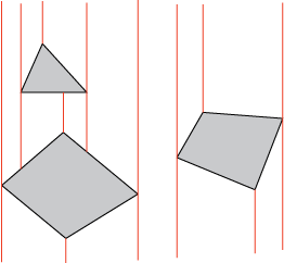
One approach to building this decomposition algorithmically would be to draw a vertical line through each vertex. Find the intersections of these vertical lines with the boundaries of the obstacles. Cells each have two vertical boundaries, and up to two boundaries (the upper and lower) that are formed from segments of the obstacle boundaries. The cells are possibly-open quadrilaterals. We can see from the shape of the cells that if two cells touch along an edge, any path from one cell to the other through that edge will not leave those cells, so two free cells can be easily connected by a path.
The number of cells depends on the number of vertices, rather than on some arbitrary resolution.
Visibility graphs
The next approach relies on an idea which may seem obvious: if there is a path between the start and goal, then there is at least one shortest path between the start and goal. This is not true for all motion problems, but it does hold for polygonal obstacles in the plane. It turns out that the structure of the shortest paths is quite simple, and there is a finite number of candidate shortest paths. We therefore restrict our search only to candidate shortest paths.
Without obstacles, shortest paths are straight lines. It turns out that in any space, shortest paths have three components:
Pieces that are in free space, and are shortest in free space. (e.g, lines)
Pieces that follow boundaries of obstacles
Jump points (places where the path jumps from type #1 to type #2 or vice versa.
For our problem, we have 1) straight lines in free space, 2) straight lines along the boundary of the obstacles, and 3) jumps (at vertices).
One way to think about this is the following. Consider any path from the start to the goal. If we shorten that path as much as possible without breaking through the boundary of an obstacle, there will be no curves in the resulting path, but only line segments. The endpoints of these line segments will be the start, the goal, or a vertex of a polygonal obstacle.
So draw a graph that connects the start to every other vertex (and the goal). Keep lines that do not go through obstacles. Now connect every vertex to every other vertex, and to the start and goal. The remaining graph structure must contain the shortest path, and we can search for it, using nodes at vertices and at start and goal.
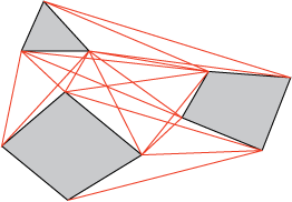
If we connect all pairs of vertices (treating the start and goal as vertices), we will have a graph with \(O(n^2)\) edges. Some of those edges pass through obstacles; we remove such edges, leaving what is known as the visibility graph. (We say adjacent vertices in the graph can “see” each other, since they are connected by line segments that do not intersect obstacles.)
Skeletons; Voronoi diagrams
Visibility graphs reduce the dimensionality of the search space from \(R^2\) to a graph that represents the connectivity of the space; the dimensionality of this graph is 1, since it is made up of connected line segments. The graph is connected if and only if the free space of configurations is connected.
We call a one-dimensional structure that is connected if and only if the embedding space is connected a skeleton of the space.
A visibility graph is a skeleton of a planar space with polygonal obstacles. If the obstacles are not polygonal, it is not obvious how to construct the visibility graph. It turns out that an application of Snell’s law describes the tangents to smooth obstacle boundaries, but we will not go into the details.
There are other ways to generate a skeleton of a two-dimensional space. One example is the Voronoi diagram. Label each point in the free space by which obstacle it is closest to. It turns out that the boundaries of these regions form a skeleton of the space.
Higher dimensions
Things get trickier in higher dimensions. First, consider shortest paths among polyhedral obstacles in three dimensions. The paths are still made up of line segments, but the line segments may contact edges of the polyhedra rather than the vertices, so the shortest path may not be contained on the visibility graph of the vertices. (Consider taking a path around a cube from start to goal. Think of the path as a string, and tighten it. There is no reason to expect that it contacts the cube only at vertices!)
The Voronoi regions are now 3D cells, and their boundaries are surfaces. No skeleton to be found here, either. One idea is to build skeletons on those surfaces, and create a hierarchy for path planning.
Exact cell decompositions are also hard in higher dimensions – it tends to be difficult to represent boundaries of the obstacles, and the boundaries may be concave.
The curse of dimensionality
The number of nodes in a graph used for motion planning tends to scale exponentially with the dimensionality of the space. For example, consider grid cell decomposition, which is straightforward to implement in any dimension. With even a coarse division of cells, the number of cells explodes by the time we reach even five or six dimensions.