Mobile robot motion

We have been discussing the differential kinematics of robot arms, that relate the motion of joint velocities and the motion of an end-effector. The Jacobian matrix converts from joint motions \((\dot \theta_1, \dot \theta_2, \dot \theta_3, \ldots)\) to a workspace velocity, perhaps \((\dot x, \dot y)\) for a planar robot.

We derived the Jacobian matrix for amrs by taking a time derivative of the forward kinematics equation. For mobile robots, the situation is trickier. We don’t have a description of forward kinematics; the location of the robot could be anything, regardless of the angle of the steering wheel or the angles of the wheels. Yet we would still like to see how the robot moves if the wheels are given certain velocities, or the steering angle is set to some particular value. We will derive the differential kinematics more directly, by reasoning about velocities.

We will find that the situation for some robots, steered cars and differential drives, is most like case (3) above: there will be fewer controls (for example, wheel speeds) than configuration variables of the robot. As a result, these robots cannot move in arbitrary directions. A steered car cannot drive sideways.

Here are a few different robot types.

A differential drive

An omni-directional robot: Rovio

Segways are another example of differential drives, as are simple wheelchairs. Tanks are differential-drives with treads.

Steered cars

You know what a steered car looks like. Let’s start with a simplified car, with one front wheel: a tricycle.

The configuration of the robot is given by specifying the location and angle of the robot frame relative to some world frame,

\(q = \begin{pmatrix} x \\ y \\ \theta \end{pmatrix}\)

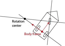
There are some constraints on the robot motion. We can describe the motion of a rigid body using a rotation center, about which the entire rigid body rotates, and an angular velocity about that rotation center.

Consider the rear wheels first. If we assume that the wheels cannot slip sideways, they must instantaneously be moving in the direction they are pointing. Any rotation center along the line colinear with the rear axle will correspond to motion of the wheels in this direction. Any rotation center not along this line would cause the wheels to move at least partially in a sideways direction.

A similar constraint applies to the front wheel. The rotation center must be along a line through the front axle. However, the front wheel can be steered, so the direction of this line can be changed. There are some limits; the front wheel should not be turned to be perpendicular to the rear wheels. A limit on the angles of the front wheels corresponds on a limit to how close the rotation center may be to the robot. Specifically, the distance of the rotation center from the center of the robot frame is proportional to \(v/ \omega\), where \(v\) is the magnitude of the tangent vector along the robot trajectory, and \(\omega\) is the angular velocity. So there is a constraint that

\(|\frac{v}{\omega}| \ge k\),

where \(k\) is a constant related to the maximum steering angle.

We now have the velocity “controls” \(v\) and \(\omega\). How do these controls relate to motion of the robot? We have the equations:

\(\begin{pmatrix}\dot x \\ \dot y \\ \dot \theta \end{pmatrix} = \begin{pmatrix}\cos \theta \\ \sin \theta \\ 0 \end{pmatrix} v + \begin{pmatrix} 0 \\ 0 \\ 1 \end{pmatrix} \omega\)

The vectors on the right hand side of the equations are vectors, and they are defined over the configuration space. Give a new \(\theta\) and you get a new vector; these vectors therefore each describe a field of vectors over the configuration space. We therefore call each of the two vector functions of \(q\) a control vector field, since each is associated with a particular control.

You could also write the control vector fields as columns of a matrix:

\(\begin{pmatrix}\dot x \\ \dot y \\ \dot \theta \end{pmatrix} = \begin{pmatrix}\cos \theta & 0\\ \sin \theta & 0 \\ 0 & 1 \end{pmatrix} \begin{pmatrix} v \\ \omega \end{pmatrix}\)

Ackerman steering

Wikipedia has a nice simple article on Ackerman steering. The two front wheels are not parallel, since otherwise their motions would be inconsistent with a rotation of the car around a rotation center. Here’s a picture from the Wikepedia article:

Notice how the four-bar linkage maintains the proper relationship between wheel angles; essentially, the closed-chain linkage is being used as a device for “computation”: an input angle for one wheel maps to an output angle for the other wheel.