Constraints and frames

We will need ways to describe mechanical systems so that we can reason about them, or write algorithms to control them. The word system is used in many ways in the robotics literature, but the definition we will use is

System: A set of particles.

In a physical system, each particle has a location in a plane, described by two real numbers, or in three-dimensional space, described by three real numbers. We say that the particles are embedded in \(R^2\) or \(R^3\). We define the configuration of the system:

Configuration: The location of every particle in the system.

The particles may be constrained to lie on a curve, or on a surface. There may also be other constraints; for example, the particles might all be part of a rigid body, so that their locations are not independent.

Configuration space: The set of all possible configurations of the system.

Degrees of freedom: The independent ways in which the configurations of a system can change.

This definition of degrees of freedom is accurate, but vague. What does “independent” mean in this context? What does “ways” mean? In some cases a more precise definition is possible; we will see this by the end of the lecture.

Let’s look at a concrete example. Consider a single particle in the plane. It takes two numbers to represent the particle’s location, so the particle has two degrees of freedom. How about a system of two particles that can move independently? Four numbers are needed, so the system has four degrees of freedom.

What happens if there are constraints on the motion of the particles? Consider a system made up of two particles, constrained so that the distance between the particles is one. (One what? It could be one meter, or one inch, or one micron. Let’s agree to always use the same units for everything, so that we can omit writing the units.) We could represent the configuration of the system using four numbers, \((x_1, y_1, x_2, y_2)\), the Cartesian coordinates of each point.

However, not all choices of four coordinates are consistent with the constraint

\((x_2 - x_1)^2 + (y_2 - y_1)^2 = 1\)

This constraint removes one degree of freedom, so this system has three degrees of freedom. How can we tell? If you knew three of the values of the coordinates (for example, \(x_1, y_1, y_2\)), then the last coordinate (\(x_2\)) would be “almost” determined. Notice that although there are actually two possible solutions for \(x_2\), no motion is possible between those points; a set of discrete points has dimension zero. So, since three numbers and the constraint remove the possibility of continuous motion, this system has three degrees of freedom.

Let’s imagine that we still use four numbers to represent the configuration of this two-point system. The possible configurations are then a three-dimensional surface embedded in \(R^4\). This surface is smooth everywhere, and local motion on the surface is possible everywhere, while preserving the rigid-body constraint.

Trajectories in configuration space

Every point on the configuration space surface corresponds to a configuration of the system. For example, the coordinate \((0, 0, 1, 0)\) on this surface would indicate that one of the particles in the system is at the origin, and the other is on the positive x axis at distance 1. We could describe a smooth continuous motion of the rigid body by a curve that lies within the configuration space, parameterized by time: \(( x_1(t), y_1(t), x_2(t), y_2(t) )\), with \(t \in [0, T]\), where zero is the start time, and \(T\) is the end time.

We distinguish between a path and a trajectory.

Path: A continuous curve on the configuration space.

Trajectory: A continuous curve on the configuration space parameterized by time.

There are some formal mathematical terms to describe the relationship between a path and a trajectory: a trajectory is a parameterization of a path, and the image of a trajectory over time is a path. A path simply tells where the particles of a system might go; a trajectory also tells us information about the velocity of the system and the time at which it gets to each point.

Topology of configuration spaces

We have said that the configuration space is a surface. Surfaces may be smooth or nonsmooth, differentiable or not, connected or not. A manifold is a special type of surface that is locally similar to \(R^d\). That is, at every point on the surface, it is possible to attach a local coordinate system with \(d\) dimensions. If the configuration space is a manifold, there is a precise way to count the degrees of freedom of a system: the number of degrees of freedom is equal to the dimensionality of the manifold. Most of the configuration spaces we will see will be manifolds, but there will be exceptions.

The surface of a sphere is a 2-manifold; at each point you can attach a local two-dimensional coordinate system. For example, at most places on the sphere you could use latitude and longitude as your coordinates. However, you should choose something else in the neighborhood of the north pole, since all longitudes describe the same point if the latitude is 90. That’s why we say “local” two-dimensional coordinate system.

The plane is also a 2-manifold (just choose coordinates x and y everywhere, for example). However, there is an interesting difference between these manifolds: the plane is infinite, while the surface of the sphere is finite. Neither manifold has a boundary. If you “keep going” on the surface of the sphere you might end up somewhere you’ve been before; this won’t happen in the plane. The study of which points are adjacent to other points is called topology. There are a few standard surface shapes that we will see over and over.

First, the one-dimensional surfaces. The real number line \(R\) is infinite and does not loop back on itself. On the other hand, the unit circle has one loop and is finite; we call the unit circle \(S^1\). What about more complicated curves? If the curve is infinite and does not cross itself, then we can establish a one-to-one correspondence between points on the curve and points on the real line \(R\); we say that the curve has the topology of \(R\). If the curve has a single loop, and can be continuously deformed into a circle without changing the adjacency relationship between any points, the curve has the topology of a circle, \(S^1\). How about a figure-eight? There are two loops. In fact, since the tangent space is not similar to either \(R^1\) or \(R^2\) at the junction point, the figure eight is not even a manifold. Maybe there is a standard name for the topology of a figure eight, but I do not know it.

Let’s think about two-dimensional manifolds. One example is \(R^2\). It is infinite in all directions and contains no holes. Another is \(S^2\), the surface of a sphere. How about an infinite cylinder? In one direction, you can move around the outside of the cylinder, coming back to where you started. In another direction, you move off towards infinity. We say that the topology is \(R \times S^1\). The \(\times\) symbol is called the Cartesian product, and it means that for each element from one space, there is associated an entire space of the second type. We are already familiar with the Cartesian product: \(R^3\) is the same as \(R \times R \times R\).

The d-dimensional unit sphere is given the symbol \(S^d\). Remarkably, the topology of \(S^d\) is not \(S^1 \times S^1 \times S^1\ldots S^1\) for \(d \ge 2\). Consider \(S^2\). You might choose to describe locations on the sphere by latitude and longitude. For most latitudes, there is in fact an entire circle of longitudes, so we might be tempted to say that the topology is \(S^1 \times S^1\). However, at two latitudes (at the north and south poles), there is not an entire ring of longitudes.

So what shape does the topology \(S^1 \times S^1\) describe? For each point on a torus, there are two types of circles: one that goes around the rim of the donut, and one that goes all the way around the hole in the center of the donut. There is no degenerate pole, as there is for the unit sphere. In general, the topology of the d-dimensional torus is the Cartesian product of d circles. This is more than a mathematical curiosity – we will see that many robot arms have configuration spaces with the topology of a torus.

Let’s return to the example of a 2-particle rod of unit length in the plane. We said that the configuration space was embedded in \(R^4\), and there was one constraint, so the dimensionality of the configuration space was 3. Although we have not shown this, it also turns out that the configuration space is a manifold. What is the topology of this manifold? There are two directions of translation, and a rotation. This indicates that the topology of the configuration space is \(R^2 \times S^1\). We will go into more details when we discuss rotations and translations.

Constraint counting

For a complicated system, it can be daunting to count the independent degrees of freedom. The most reliable method is based on the observation that a constraint typically removes a single degree of freedom. For example, our 2-particle rigid body of length one had the constraint

\((x_2 - x_1)^2 + (y_2 - y_1)^2 = 1\).

If the length of the rod were able to vary freely, then the two particles could move independently. The constraint removes this dimension, length, so the rigid body has three degrees of freedom. What if we added another constraint? For example,

\(x_1= 0\)

Then the rigid body could slide along the y axis and rotate, but could not translate in the x direction. We have removed one more degree of freedom. How about one more constraint?

\(y_1 = 0\)

Now the rod is pinned to the origin, and can only rotate. By adding three constraints, we have reduced the degrees of freedom of the two-particle system from four (\(R^4\)) to one (\(S^1\)). It can be tricky to figure out which degrees of freedom remain after applying several constraints, but counting how many degrees of freedom remain is easy: just subtract one degree of freedom for each independent constraint. (We will see later what is meant by independent.)

Configuration spaces for rigid bodies

Armed with constraint-counting, we are now ready to think about the degrees of freedom for systems that are more complicated than just two points. Many of the objects we study in robots are approximately rigid. Consider a system of \(n\) particles in the plane. If unconstrained, each of the \(n\) particles has two degrees of freedom, so the system has \(2n\) degrees of freedom in total.

A rigid body has constraints that maintain the distance between each pair of particles. There are n choose 2 pairs of particles, so a naive application of constraint counting would suggest that a rigid body has 2n - choose(n, 2) degrees of freedom. This would imply that a system with 10 particles had \(2 * 10 - 45 = -25\) degrees of freedom. Something is wrong.

The problem is that many of the constraints in the rigid body are redundant. If we had two particles, and one constraint between them (as in our example system), there would be \(2 * 2 - 1 = 3\) degrees of freedom, which is what we expect. Since there is only one constraint, it is clearly not redundant. Now imagine adding one additional particle. We need to attach it to each of the previous particles, requiring two additional constraints. So we have three particles and three constraints; \(2 * n - 3 = 3\) degrees of freedom, still. Now let’s add a fourth particle. We want the distance to each of the particles in the triangle already formed to remain constant, but we can do this by adding only two constraints, specifying the distance to only two of the previous particles. We now have \(n = 4\) and there are 5 constraints, so we still have three degrees of freedom. Each additional particle requires only two constraints to fix it to the current rigid body, so in general, the rigid body in the plane has three degrees of freedom.

Parametrized configuration space

It would be inconvenient if we had to write down the location of every particle in a rigid body to describe the configuration. Instead, we are likely to choose a reference point on the body, and describe the configuration of the body by stating the location of that coordinate, and the orientation of the body with respect to some initial orientation.

Consider a simple example of a particle in \(R^2\) constrained to lie on a unit circle. The configuration space has one dimension; there is one degree of freedom. The topology of the configuration space is \(S^1\). We could express the configuration using two numbers and a constraint:

\(x = (x_1, x_2) \in R^2\)

\(x_1^2 + x_2^2 = 1\)

or we could use a single number \(\theta \in [0, 2\pi)\) to describe the angle of of the particle with respect to the horizontal. The second representation is convenient in that it uses only one number instead of two. This is called a ‘reduced-coordinate’ description of the configuration. If the number of coordinates matches the number of degrees of freedom (i.e. no additional constraints are needed) then it is a minimal coordinate representation of the system.

Minimal coordinates are not always the best choice. It may be difficult to determine what the minimal coordinates are, and when we are thinking about the motion of the system, we may still need to worry about the fact that the particles are really following a curve, moving along a surface. There are problems both of topology and geometry. For example, think about a point body in \(R^3\) constrained to move on a sphere. You could use the latitude and longitude as minimal coordinates: \(q = (\theta_1, \theta_2)\). Let’s say you’d like to sample the surface of the sphere. If you sample the latitudes and longitudes, you will get many many more points near the north and south pole than anywhere else, which is probably not what you wanted. The fact that all longitudes are the same at the north and south poles is also going to cause trouble with numerical computations involving velocities near the poles. If you are very close to the north pole, even a slow walk east is going to change your longitude very fast. We will see these problems again when we look at Euler-angle representation of rotations in 3D.

Even so, minimal coordinates are the most typical way to represent the configuration of a mechanical system. We assign one coordinate for each degree of freedom, and use a vector of numbers (by convention, this vector is named \(q\)) to describe the configuration. For example, the configuration space for a rigid body in the plane has the topology $ R^2 S^1$, so it is common to take \(q = (x, y, \theta)\), which describes the location and orientation of the body with respect to some world frame. (We will look at frames more closely in the next few lectures.)

A revolute joint allows one degree of rotation, so the configuration of a joint might be represented by an angle \(\theta\). A planar robot arm with three revolute joints connected serially might have the configuration described by \(q = (\theta_1, \theta_2, \theta_3)\); the topology of the configuration space is \(S^1 \times S^1 \times S^1\).

The minimal coordinates are parameters that describe a location in configuration space: that is, the coordinates can be used to determine the location of every particle in the system. As the parameters change, the configuration of the system changes. There may be many different possible choices of coordinate systems to describe the same configuration space; we call such a choice a “parameterization” of the space.

Definition of a rigid body

A rigid body is a system of particles with the constraint that the distance between any pair of particles is fixed. No physical body is entirely rigid, but rigid-body models are good enough for many purposes. There are situations where rigid-body models do not work as we would like; for example, during collisions, the forces generated depend on deformations of the bodies.

Displacements

A displacement is a transformation of a system that maintains the distance between every pair of points in the system. Rigid bodies are therefore systems for which we only allow displacements.

There are two special types of displacements:

A rotation is a displacement that leaves a single point (called the center of rotation) fixed. Notice that there’s no reason that the point has to a particle in the system; the fixed point could be anywhere. Another thing to notice is that this definition of rotation applies in any number of dimensions.

A translation is a displacement where all points move along parallel lines.

There are displacements in 3D that are neither pure translations nor pure rotations, but it turns out that they are just combinations of translations and rotations. In fact, given a displacement, you choose an arbitrary point in space, and get that displacement by a rotation that leaves that point fixed, followed by a translation. (Intuition. Think about a rigid body in two configurations. Choose a point O. Rotate the body however you like, but keeping the distance of every point on the rigid body the same distance from O. You can eventually get he body to be in the same orientation as the goal configuration. Then you’ll have to do a translation to get the body into the right place. A formal proof can be found in the Mason text.)

All displacements in the plane are pure rotations (or translations)

A displacement can be viewed as a translation composed with a rotation about any point. However, if you choose that point carefully in the plane, you can get rid of the translation component.

Here’s an experiment to try for yourself. Cut out a “rigid body” from a piece of paper; any shape you like. Mark two different points on the body, A and B. Outline the body on a piece of “background” paper, and mark the two points also. Move the body from one configuration to another – this motion is a displacement. Outline the body in its new configuration on the background paper, and mark the two points in their new configurations, A’ and B’. Notice that the center of rotation, if it exists, must be on the perpendicular bisector of the segment AA’; draw this bisector. The center of rotation must also be on the perpendicular bisector of BB’; draw this bisector. The center of rotation must be at the intersection of the two bisectors you just drew.

But what if the two bisectors are parallel, and don’t intersect? That’s a pure translation. It doesn’t appear to leave any point fixed. However, if the motion were almost a pure translation, the lines would intersect, just very far away. As we get closer and closer to translation, that intersection moves towards infinity. In projective geometry, we are allowed to have points at infinity – a translation is therefore a rotation about a point at infinity, in a particular direction.

The fact that displacements in the plane are pure rotations is a special case of the fact that all displacements in space are screws (Chasle’s theorem). A screw is a rotation about an axis, combined with a translation parallel to that axis. There is a proof of Chasle’s theorem in Mason.

Reuleaux’s method for analyzing planar rigid-body grasps

The fact that all displacements in the plane are pure rotations allows graphical methods for analysis of rigid body motion. For example, consider grasping a rigid body with n point fingers. Assume that the fingers are frictionless, and apply unilateral forces (they push, but do not pull). How many fingers need to be placed around the boundary of a planar rigid body to immobilize it?

Here is a triangular rigid body being grasped by three fingers (one red, one green, and one blue).

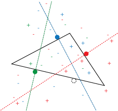
Is the body immobilized? What if we add a finger at the location shown by the dotted circle? First, consider the way a single finger restricts the motion of the body. For example, the red finger. Any displacement can be described by a rotation center, and a distance and direction to rotate around that rotation center. So pick a rotation center. Notice that either the finger prohibits clockwise (negative) rotations, or prohibits counterclockwise (positive) rotations, unless the rotation center is on the line through the finger parallel to the normal.

So we can label each rotation center as allowing positive or negative rotations. The red + and - signs show the allowed rotation for rotation centers at various locations.

Now consider the blue finger. Each rotation center may be similarly positive, or negative. What if a rotation center is positive for the red finger, and negative for the blue? That means that rotation in either direction will cause a collision with at least one finger, so these rotation centers are not possible.

We add each additional finger, labeling rotation centers, and removing regions where the signs conflict. If, at the end, the entire plane of rotation centers has been removed, the object is in an immobilizing grasp.