Lab Assignment 3: Sorting it all out
Computer science is about a lot more than handling data, but computers are still a very useful tool for working with large amounts of data. Scientific experiments in biology, chemistry, physics, and psychology can generate huge numbers of measurements. In economics, business, or politics, data can be generated by everything from stock prices, to poll results, to voting records of congresspeople. In this lab, you’ll read data from a file, organize that data using a class, write an algorithm to manipulate the data, and visualize your result.
You saw the selection sort algorithm, insertion sort, and merge sort. One part of this assignment will ask you to implement yet another sorting algorithm: quicksort. Quicksort has a worst-case running time of O(n2) (worse than merge sort), but the worst case for quicksort occurs rarely—rarely enough that on average, it runs in O(nlog n) time. Quicksort has two advantages over merge sort: the constants are better, and quicksort runs “in place”: no temporary lists have to be created, and so very little additional memory is required to quicksort.
Now, you might ask why you need to implement quicksort when Python has a sorting method built in and when you’ve already learned three other sorting algorithms. That’s a fair question, but if the professors who taught the Python designers had let them skip sorting, we wouldn’t have such a nice built-in sort function in Python. I won’t let you skip learning how to sort, either!
In this lab assignment, you will read in a text file in which each line describes a world city, store the information about each city in its own object within a list, sort the list using quicksort, write the results out to a file, and display part of the output file in a visualization on a world map.
Checkpoint: File input and output
For the checkpoint, you just need to read in the file of world city information, store the information about each city into its own City object within a list, and write out each object (converted to a string) to a file. You don’t need to sort anything, and you don’t need to do the graphics.
Checkpoint step 1: Define a City class
Your first job in the checkpoint is to define a City class in a file named city.py. Each City object will need instance variables to store the following information:
- The city’s country code, which is a two-letter string.
- The city’s name, which is a string.
- The city’s region, a two-character string.
- The city’s population, which is an int.
- The city’s latitude, which is a float.
- The city’s longitude, which is also a float.
You need to write only two methods in the City class. The __init__ method does the usual: it takes six parameters (plus self) and stores each in the appropriate instance variable. The __str__ method returns a string consisting of the city’s name, population, latitude, and longitude, separated by commas and with no spaces around the commas. The string returned by your __str__ method should be exactly as specified here, because your section leader will compare your resulting file with one that is I’ve prepared, and the two files need to be identical in order to give you full credit for the checkpoint.
For example, here’s the string that __str__ should return for a particular town in New Hampshire:
Hanover,11222,43.7022222,-72.29Notice that the country code and region do not appear in the string returned by __str__.
Checkpoint step 2: Read in and parse the input file
The input file is in world_cities.txt. Download this file, and drag it into your PyCharm project. This file has 47913 lines. Each line has information about a world city, specifically the six attributes you’ll store in the City object, but of course represented textually. These attributes are separated by commas without surrounding spaces. We call such a file a CSV file. (CSV is short for “comma-separated values.”) Here’s the line of the world_cities.txt file for that town in New Hampshire:
us,Hanover,NH,11222,43.7022222,-72.2900000Here, the country code is us, the city name is Hanover, the region is NH, the population is 11222 (Dartmouth students living on campus don’t count in Hanover’s population), the latitude is 43.7022222, and the longitude is –72.2900000. You already know how to read in a file, line by line. But if you forgot, see the notes from Chapter 9. But how can you process this line? Python makes it pretty easy.
To separate text at a particular delimiter character, call the split method on the string. It returns a list of the strings that, concatenated with the delimiter added in, gives you back the string. This idea is best shown by an example:
s = "a man, a plan, a canal,"
clauses = s.split(",")
print clauses
prints
['a man', ' a plan', ' a canal', '']Note that every character other than the commas becomes part of one of the strings in the list. Not only do the spaces after the first two commas become part of strings in the list, but we also get an empty string at the end. Why? Because the string s ends with a comma, and so the split method gives back the empty string after the comma.
You can use any character as the delimiter, and the default is a space character. More examples:
s = "Roll out the barrel"
words = s.split()
print words
prints
['Roll', 'out', 'the', 'barrel']And
s = "commander--in-chief"
parts = s.split("-")
print parts
(there are two hyphens between commander and in) prints
['commander', '', 'in', 'chief']Again, note the empty string caused by two delimiters in a row.
To strip away whitespace from the beginning and end of a string, call the strip method on the string:
s = "  The thousand injuries of Fortunato I had borne as best I could, \n"
t = "|" + s.strip() + "|"
print t
prints
|The thousand injuries of Fortunato I had borne as best I could,|I put the vertical bar characters in so that you could see where the string returned by the call s.strip() begins and ends.
Although each line of world_cities.txt begins with a non-whitespace character, each line ends with a newline, and newline is a whitespace character. Therefore, you will want to call strip on each line of the file and then call split to separate the information by the commas.
Once you have a list of information in a particular line of the file, you can send that information into the City constructor. Since split gives you a list, you can just index into that list for each item. Remember that some of the instance variables in a City object are not strings, and so you will have to convert these strings to the appropriate types.
The City constructor will give you back, as you undoubtedly know, a reference to a City object. You should append that reference to a list that you’re building up. When you’re done, the list should comprise 47913 references to City objects, one for each line in world_cities.txt.
Checkpoint step 3: Write the output file
Once you have the list of references to City objects and you have the __str__ method of the City class defined, all you need to do now is create a file named cities_out.txt and write one line to it for each City object. The line for each city should contain the string returned by calling str on the corresponding City object. Because the __str__ method inserts commas, cities_out.txt will be a CSV file. You’ll need to add the newline for each city. When you’re done, your cities_out.txt file should have 47913 lines. The first five and last five lines of cities_out.txt should be
Andorra La Vella,20430,42.5,1.5166667
Canillo,3292,42.5666667,1.6
Encamp,11224,42.5333333,1.5833333
La Massana,7211,42.55,1.5166667
Les Escaldes,15854,42.5,1.5333333
...
Redcliffe,38231,-19.0333333,29.7833333
Rusape,23761,-18.5333333,32.1166667
Shurugwi,17107,-19.6666667,30.0
Victoria Falls,36702,-17.9333333,25.8333333
Zvishavane,79876,-20.3333333,30.0333333
Because the format of this file is tightly constrained, and because you’ll be creating the file from world_cities.txt, your section leader has an automated tool to check that your cities_out.txt file is correct. It should match a file that your section leader has, in every single byte.
For the checkpoint, submit your code and your cities_out.txt file.
Quicksort
Once you have done the checkpoint, you will need to sort the list of City objects according to various criteria. You will use the quicksort algorithm to sort.
Like merge sort, quicksort is recursive. As in merge sort, the problem is to sort a sublist the_list[p : r+1], which consists of the items starting at the_list[p] and going through the_list[r]. (Recall again that in Python’s slice notation, the number after the colon is the index of the first item not in the sublist.) Initially, p equals 0 (zero) and r equals len(the_list)-1, but these values will change through the recursive calls.
Important note: In several places in this lab writeup, we use Python’s sublist notation, such as the_list[p : r+1]. We use this notation only to indicate the range of indices you should be working with. Do not use this sublist notation in your program. Why not? Because it will make a copy of the sublist of the_list, and if you change values in a sublist you create using sublist notation, the values in the_list itself will not change.
Divide: Choose any item within the sublist
the_list[p : r+1]. Store this item in a variable namedpivot. Partitionthe_list[p : r+1]into two subliststhe_list[p:q]andthe_list[q+l : r+1](note thatthe_list[q]is in neither of these sublists) with the following properties:- Each item in
the_list[p:q](the items in positions p through q − 1) is less than or equal to the value ofpivot. - The value of
pivotis inthe_list[q]. - Each item in
the_list[q+1 : r+1](the items in positions q + 1 through r) is greater than the value ofpivot.
- Each item in
Conquer: Recursively sort the two sublists
the_list[p:q]andthe_list[q+l : r+1].Combine: Do nothing! The recursive step leaves the entire sublist
the_list[p : r+1]sorted. Why? Because the subliststhe_list[p:q]andthe_list[q+l : r+1]are each sorted, each item inthe_list[p:q]is at most the value ofpivot, which is inthe_list[q], and each item inthe_list[q+1 : r+1]is greater thanpivot. The sublistthe_list[p : r+1]can’t help but be sorted!
The base case is the same as for merge sort: a sublist with fewer than two items is already sorted.
Partitioning
It doesn’t take much insight to see that all the work in quicksort occurs in the partitioning step, so let’s see how to do that. You will write a function with the following header:
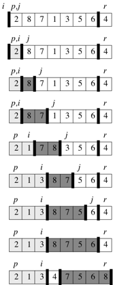
def partition(the_list, p, r, compare_func):This function should partition the sublist the_list[p : r+1], and it should return an index q into the list, which is where it places the item chosen as the pivot. As a running example, we’ll suppose that the current sublist to be sorted is [2, 8, 7, 1, 3, 5, 6, 4], so that the_list[p] contains 2 and the_list[r] contains 4.
First, we need to select an item as pivot. Let’s always select the last item in the sublist, that is, the_list[r]. In our example, we select 4 as the value of pivot. When we’re done partitioning, we could have any of several results. Here are three of them:
[3, 2, 1, 4, 7, 8, 6, 5]
[1, 3, 2, 4, 8, 7, 5, 6]
[2, 1, 3, 4, 6, 8, 5, 7]
Several more are possible, but what matters is that 4 is in the position it would be in if the sublist were sorted, all items before 4 are less than or equal to 4, and all items after 4 are greater than 4.
We want to partition the sublist efficiently. (Remember that we’re in the part of the course where not only do we want right answers, but we want to use resources—especially time—parsimoniously.) If the sublist contains n items, we might have to move each one, and so O(n) time for partitioning an n-item sublist is the best we can hope for. Indeed, we can achieve O(n) time. This picture gives you an idea of how:
You can also look at this PowerPoint.
The idea is to loop through the items in the_list[p:r] (which does not include the_list[r], the value of pivot.) Maintain two indices, i and j, into the sublist:
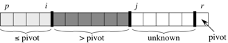
At the start of each loop iteration, for any index k into the sublist:
- If p ≤ k ≤ i, then
the_list[k]≤pivot. - If i + 1 ≤ k ≤ j − 1, then
the_list[k]>pivot. - If j ≤ k ≤ r − 1, then we have yet to compare
the_list[k]withpivot, and so we don’t yet know which is greater. - If k = r, then
the_list[k]equalspivot.
Start with i = p − 1 and j = p. There are no indices between p and i, and there are no indices between i + 1 and j − 1, and so the above conditions must hold: all indices k between j and r − 1 have yet to be compared with pivot. Set pivot = the_list[r] to satisfy the last condition.
Each iteration of the loop finds one of two possibilities:
the_list[j]>pivot: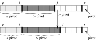
All you need to do is increment j. Afterward, condition 2 holds for
the_list[j-1], and all other items remain unchanged.the_list[j]≤pivot: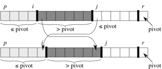
In this case, you need to increment i, swap the values in
the_list[i]andthe_list[j], and then increment j. Because of the swap, we now have thatthe_list[i]≤pivot, and condition 1 is satisfied. Similarly, we also have thatthe_list[j-1]>pivot, since the item that was swapped intothe_list[j-1]is, by condition 2, greater thanpivot.
The loop should terminate immediately upon j equaling r. To be clear: the last time that the loop body should execute is for j = r − 1. The loop body should not execute when j = r.
Once j equals r, every sublist item before the_list[r] has been compared with pivot and is in the right place. All that remains is to put the pivot, currently in the_list[r] into the right place. Do so by swapping it with the item in the_list[i+1], which is the leftmost item in the partition known to be greater than pivot. (If the greater-than partition happens to be empty, then this swap should just swap the_list[r] with itself, which is fine in this case.)
Your partition function should return to its caller the index where it has placed pivot. Within partition, that’s index i + 1.
The function compare_func will be one that you write and pass in. It takes two parameters, say a and b, and it returns True if a compares as less than or equal to b, and it returns False if a compares as greater than b. For example, the call compare_func(3, 5) should return True, the call compare_func(7, 5) should return False, the call compare_func(5, 5), should return True, the call compare_func("Tallahassee", "Tokyo") should return True, and the call compare_func("Boise", "Bismarck") should return False. Your partition function should call compare_func to compare each sublist item with pivot.
You can write your own functions that take a function as a parameter. Here’s an example:
from string import lower

def do_it(compare_func, x, y):
    if compare_func(x, y):
        print x, "is less than", y
    else:
        print x, "is not less than", y

def compare_ints(a, b):
    return a <= b

def compare_strings(a, b):
    return lower(a) <= lower(b)

do_it(compare_ints, 5, 7)
do_it(compare_strings, "Dartmouth", "Cornell")
The call do_it(compare_ints, 5, 7) passes the function compare_ints into do_it as the first parameter, and so in do_it, compare_func is really compare_ints. The other formal parameters of do_it are x and y, and they get the values 5 and 7, respectively. Therefore, the call compare_func(x, y) is really the call compare_ints(5, 7). This call returns True (the parameter a gets the value 5, and the parameter b gets the value 7), and so the line 5 is less than 7 is printed to the console. Next, the call do_it(compare_strings, "Dartmouth", "Cornell") passes the function compare_strings as the first parameter, and now in do_it, compare_func is really compare_strings. The formal parameter x references the string "Dartmouth", and the formal parameter y references the string "Cornell", so now when we call compare_func(x, y), we’re really calling compare_strings("Dartmouth", "Cornell"). The function compare_strings first makes copies of its parameters, but converted to lowercase (that’s what the function lower, imported from the strings module, does), and then it compares them lexically, using the ASCII character codes. Because "dartmouth" comes after "cornell" lexically, compare_strings returns False, and so the console output is now Dartmouth is not less than Cornell (which is true, because as we all know, Dartmouth is greater than Cornell).
You should implement and test your partition function before writing any other code. Make sure that it works on an arbitrary sublist of the_list, and not just on the sublist where p = 0 and $r = $len(the_list)-1. You’ll have to write the compare_func function as well, and design it so that it works on whatever data type the_list contains. You should certainly test partition on lists containing numbers and on lists containing strings.
I was able to write the body of the partition function in 10 lines of Python code (not counting blank lines and comment lines).
The quicksort function
Once you have the partition function written and tested, you should write a function with the header
def quicksort(the_list, p, r, compare_func):which sorts the sublist the_list[p : r+1], whose first item is in the_list[p] and whose last item is in the_list[r].
It should work as described above:
The base case occurs when the sublist has fewer than two items. Nothing needs to be done.
Otherwise, call the
partitionfunction to partition the sublist. The call will return an index into the sublist, indicating wherepartitionput the pivot item. Let’s say that you assign this index to the local variableq, so thatpartitionhas placed the pivot item inthe_list[q].Recursively call
quicksorton the sublist starting at indexpand going up to, but not including, indexq. Recursively callquicksorton the sublist starting at the index just pastqand going up to and including indexr.
The body of my quicksort function takes only 4 lines of Python, not counting comment lines.
The sort function
Unlike the examples from lecture, you’ll write a separate function named sort in this lab assignment. It has this header:
def sort(the_list, compare_func):It simply makes a call to the quicksort function to sort the entire list referenced by the_list.
Place the partition, quicksort, and sort functions in a single file named quicksort.py. Include in this file any other functions that your quicksort code calls, but not the comparison functions described below.
What to sort
You will sort information contained in world_cities.txt.
Produce three output files:
- cities_alpha.txt contains the list of cities sorted alphabetically.
- cities_population.txt contains the list of cities sorted by population, from most to least populous.
- cities_latitude.txt contains the list of cities sorted by latitude, from south to north.
Here are the first and last few lines of each of the files, when I ran my program:
For cities_alpha.txt:
A,1145,63.966667,10.2
A,1145,63.966667,10.216667
A Coruna,236010,43.366667,-8.383333
A Dos Cunhados,6594,39.15,-9.3
Aabenraa,16344,55.033333,9.433333
Aabybro,4849,57.15,9.75
Aachen,251104,50.770833,6.105278
Aadorf,7100,47.483333,8.9
Aakirkeby,2195,55.066667,14.933333
Aakre,295,58.1013889,26.1944444
...
Zychlin,8844,52.25,19.616667
Zykovo,1059,54.0666667,45.1
Zykovo,5365,55.9519444,93.1461111
Zyrardow,41179,52.066667,20.433333
Zyryanka,3627,65.75,150.85
Zyryanovsk,44939,49.738611,84.271944
Zyryanovskiy,896,57.7333333,61.7
Zyryanskoye,6285,56.8333333,86.6222222
Zyukayka,4556,58.2025,54.7002778
Zyuzelskiy,1311,56.4852778,60.1316667
For cities_population.txt:
Tokyo,31480498,35.685,139.7513889
Shanghai,14608512,31.005,121.4086111
Bombay,12692717,18.975,72.825833
Karachi,11627378,24.866667,67.05
New Delhi,10928270,28.6,77.2
Delhi,10928270,28.666667,77.216667
Manila,10443877,14.604167,120.982222
Moscow,10381288,55.7522222,37.6155556
Seoul,10323448,37.5663889,126.9997222
Sao Paulo,10021437,-23.533333,-46.616667
...
Girsterklaus,12,49.7777778,6.4994444
Vstrechnyy,12,67.95,165.6
Qallimiut,12,60.7,-45.3333333
Skaelingur,11,62.1,-7.0
Ivittuut,11,61.2,-48.1666667
Crendal,10,50.0577778,5.8980556
El Porvenir,10,9.5652778,-78.9533333
Schleif,8,49.9905556,5.8575
Aliskerovo,7,67.7666667,167.5833333
Neriunaq,7,64.4666667,-50.3166667
Tasiusaq,7,73.3666667,-56.05
Timerliit,7,65.8333333,-53.25
For cities_latitude.txt:
Ushuaia,58045,-54.8,-68.3
Punta Arenas,117432,-53.15,-70.9166667
Rio Gallegos,93234,-51.6333333,-69.2166667
Port-Aux-Francais,45,-49.35,70.2166667
Bluff,1938,-46.6,168.333333
Owaka,395,-46.45,169.666667
Invercargill,47287,-46.4,168.35
Woodlands,285,-46.366667,168.55
Riverton,1651,-46.35,168.016667
Wyndham,586,-46.333333,168.85
Wallacetown,638,-46.333333,168.266667
...
Kullorsuaq,408,74.5833333,-57.2
Savissivik,82,76.0233333,-65.0813889
Moriusaq,21,76.7561111,-69.8863889
Narsaq,1709,77.3025,-68.8425
Qaanaaq,616,77.4894444,-69.3322222
Qeqertat,18,77.5097222,-66.6477778
Siorapaluk,75,77.7952778,-70.7558333
Barentsburg,576,78.0666667,14.2333333
Longyearbyen,1232,78.2166667,15.6333333
Ny-Alesund,40,78.9333333,11.95
Some things you should note:
In some cases, values that you sort on might be equal. For example, there are several cities named Hanover. If you are sorting the cities alphabetically, the Hanovers may appear in any order relative to each other.
For each sorted output file, as long as the cities appear in a correct sorted order according to the criterion (alphabetical order, decreasing by population, increasing by latitude), your output is correct. The first and last lines need not match those above exactly. (Hint: In my code, I don’t bother to re-read the world_cities.txt file each time. The second sort just sorts starting from the result of the first sort, and the third sort sorts starting from the result of the second sort.)
Whatever function you use as your comparison function should take as parameters references to two
Cityobjects. The comparison function will need to access the appropriate instance variables for the comparison.When comparing city names, watch out for lowercase and uppercase letters. All uppercase letters compare as less than all lowercase letters:
"a" < "Z"evaluates toFalse. The function you use to compare city names should convert each name to either all lowercase (use thelowerfunction from thestringmodule) or all uppercase (use theupperfunction from thestringmodule) before comparing. (Choose one: either all lowercase or all uppercase.) But this conversion should be only for the purpose of comparison. Do not change the city name as stored in aCityobject. Change it only within the comparison function.When sorting by population, you want the most populous cities at the beginning of the output file. I can think of three ways to accomplish this goal. Let’s assume that you have a function
compare_population(city1, city2).compare_population(city1, city2)returnsTrueif the population of theCityobject referenced bycity1is less than or equal to the population of theCityobject referenced bycity2, and the resulting list is reversed before writing it out to a file.compare_population(city1, city2)returnsTrueif the population of theCityobject referenced bycity1is less than or equal to the population of theCityobject referenced bycity2, and the resulting list is written out to a file starting from the back end of the list.compare_population(city1, city2)returnsTrueif the population of theCityobject referenced bycity2(yes,city2) is less than or equal to the population of theCityobject referenced bycity1(yes,city1), and so the resulting list has the most populous cities first and is written out in order to a file.
Which choice do you think is the easiest to implement? (Hint: It’s the third one.)
Write the Python code that reads in the city information, sorts it according to the three criteria, and writes out the results to the three files (cities_alpha.txt, cities_population.txt, and cities_latitude.txt), along with all of your comparison functions, in a single file named sort_cities.py.
Visualizing the output
CSV files are just fine for computers, but they are not wetware-friendly. You will write a program that visualizes the output of your sorted cities.
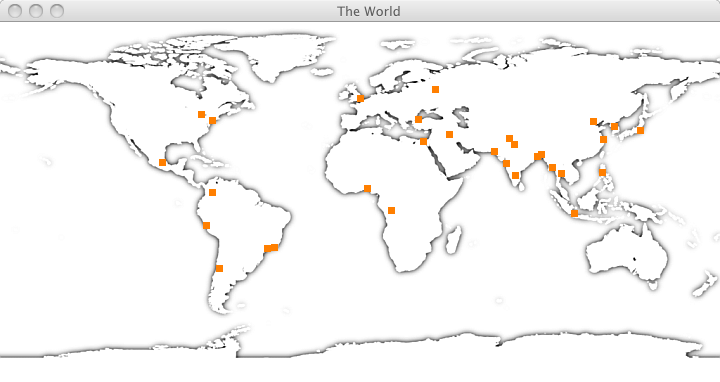
Your program will display the image file world.png:

Download this image file, and put it into your project in PyCharm. Your program will overlay the image with marks for the first n cities in an output file. For example, here’s what it looks like with small orange squares for the 30 most populous cities:
It’s easy to display this image file in a graphics window. After the window has been opened, all you need to do is
img = load_image("world.png")
draw_image(img, 0, 0)
The first parameter to draw_image is the reference to an object for the image returned by load_image. (I don’t know what kind of object this is, nor do I care. Yay, abstraction!) The second and third parameters give the x- and y-coordinates of the upper left corner of the image in the graphics window. If you are going to draw the image repeatedly, you may call load_image just once and call draw_image multiple times, as long as you have saved the reference returned by load_image.
I selected the world.png file specially because it uses linear scales for both latitude and longitude, and the (0, 0) spot is exactly in the middle of the image. This image is 720 pixels wide and 360 pixels high.
A hint for you: latitudes increase from south (bottom of the image) to north (top of the image). That’s reversed from y pixel coordinates.
But it’s not enough to just show a static image with marks for the first n cities in some order. You need to show them dynamically, in an animation. For example, you could show the first one, then the second, then the third, etc.
You may choose how you animate the cities. Show the 50 most populous cities, in order, starting from the most populous. (I’ve shown you the first 30.)
Write your visualization code in a file named visualize_cities.py.
Miscellaneous reminder
Remember to close all files that you open once you’re done reading from them or writing to them.
Grading
Checkpoint: 5 points. 3 of the 5 points are for correct behavior and testing, and the remaining 2 points are for implementation and style.
The remaining 35 points are for the final version.
Correctness: 28 points
partitionfunction: 7 pointsquicksortandsortfunctions: 6 points- comparison functions: 2 points
Cityclass: 1 point- Reading the input file and writing output files: 2 points
- Sorting alphabetically, by population, and by latitude (include all 3 output files): 3 points
- Dynamic visualization of 50 most populous cities: 7 points
Style: 7 points
- Clear design and organization: 4 points
- Good variable names, function names, and comments: 2 points
- Correct use of instance variables: 1 point
Extra credit ideas
Any extra credit work should be submitted in separate Python files. Don’t add extra credit work into your main solution code. These are just a few ideas; you are more than welcome to make up your own.
Randomized quicksort: 5 points.
The description I gave of how to partition always chooses the last item in the sublist,
the_list[r], as the pivot. Suppose that your worst enemy is supplying the input to quicksort. He or she could arrange the list so that the pivots selected inpartitionare always either the largest or the smallest items in the subarray. That would elicit the worst-case O(n2) behavior of quicksort.But you can foil your enemy by choosing a random item in the sublist as the pivot. And it’s easy! In each call of
partition, first select a random index in the range from p to r, inclusive, and swap the item at this index with the item inthe_list[r]. Then do everything thatpartitionnormally does: selectthe_list[r]as the pivot, compare all the other items in the sublist with the pivot, etc.Other maps: Up to 20 points.
The map I used has a linear scale in both latitude and longitude. Many other ways of mapping the world have been devised. Find one that has a good image and use that to map latitude and longitude.
Cool visualizations: Up to 30 points.
Come up with a cool way to visualize the cities. For example, my way of blinking each city in red, showing the name of the city, and then showing it in solid orange would be worth 10 points.
I also used boldface text when displaying the city names. I called the function
set_font_boldfrom cs1lib. Don’t forget that you can read about all the functions in cs1lib in the cs1lib User’s Guide."
What to turn in
For the final version, turn in the following:
- All of your Python code: quicksort.py, city.py (even though you turned in city.py in the checkpoint), sort_cities.py, visualize_cities.py, along with any other Python files you write.
- The output files cities_alpha.txt, cities_population.txt, and cities_latitude.txt.
- A screenshot of your visualization of the 50 largest cities once all 50 are displayed.
- Any other images or files needed to demonstrate extra credit.
Honor Code
The consequences of violating the Honor Code can be severe. Please always keep in mind the word and spirit of the Honor Code.