Lab Assignment 4: Dartmouth pathfinder
In this lab assignment, you will create a graph that models part of the Dartmouth campus, find paths from one vertex in this graph to another vertex, and display them. Here is a scaled-down screenshot from the program:
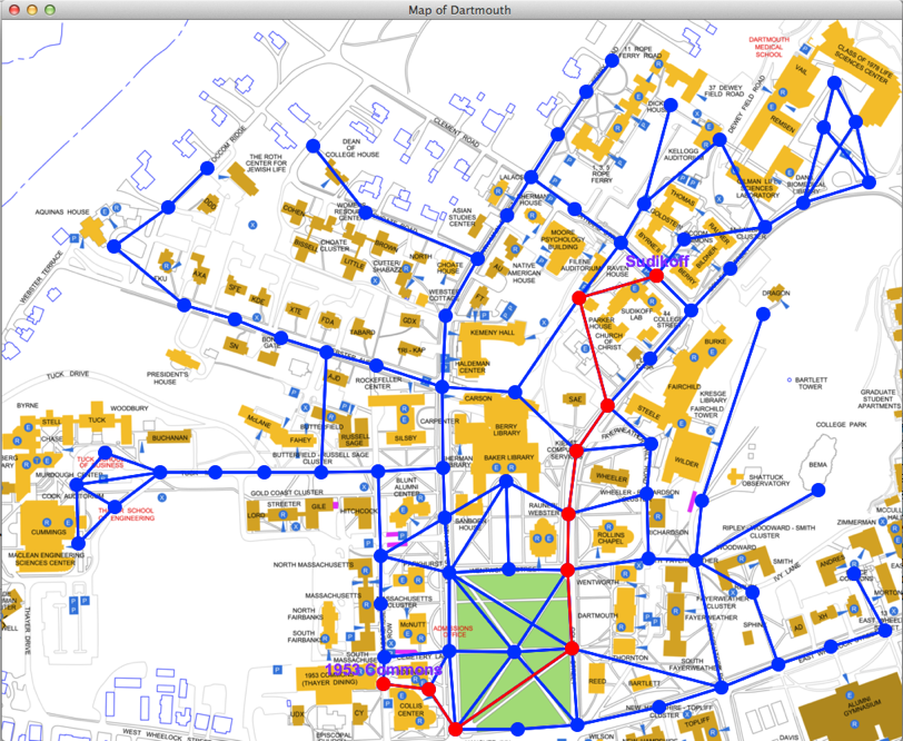
There’s a map of the Dartmouth campus. That map has a graph overlaid on top of it, with vertices drawn at their locations on the map. Many of the vertices that are close together and have a footpath between them have an edge between them.
The vertices are shown as blue circles. The edges are blue lines. To get this screen shot, I pressed and released the mouse button when it was on the vertex with a small red circle on it in front of Sudikoff. Then, with the mouse button not pressed, I moved the mouse over to a vertex near 1953 Commons. The program performed a breadth-first search on the graph and drew the resulting connecting path in red on the graph. My program also displayed the names of the starting and ending vertices, but that’s an easy extra-credit option.
I recommend that you tackle the problem in three pieces, and write one file for each piece. The checkpoint will be part of the first piece.
Load the data and create a graph data structure and a dictionary of vertices
You’ll want to create a class to hold information about each vertex. I’m calling this class Vertex, so it should be in a file named vertex.py. Creative, huh? A Vertex object should have instance variables holding its name and its x and y locations on the map. And it should have an instance variable for its adjacency list: a list (a Python list—no need to get fancy and have a linked list) of references to Vertex objects for its adjacent vertices. You’ll want to write some methods for Vertex objects; we’ll look at methods later.
After creating vertex.py, write the graph-loading function into a file called load_graph.py.
We have done the work of identifying the connections between vertices, and written a data file, dartmouth_graph.txt, which has the locations of each vertex, and the connections between each vertex. Drag this data file into your project for this lab.
Your job is to write a function load_graph in load_graph.py, which takes one parameter, the name of the data file. load_graph should create one Vertex object per line in the data file and add to a dictionary a reference to each Vertex object it creates. The Vertex references (addresses) will be the values in the dictionary, and the names of the vertices will be the keys for the dictionary. When done reading and processing all the information in the data file, the function should return the address of the dictionary, which will have information about all the vertices.
I recommend that load_graph make two passes over the data file. (You may just read it in once and save all the lines in a Python list of strings if you like.) The first pass creates all the Vertex objects, storing the coordinates in the objects, and it also creates the dictionary mapping vertex names to references to Vertex objects. But the first pass doesn’t create the adjacency lists in the Vertex objects. Why not? Because you need to have created all the Vertex objects before you can create adjacency lists. After all, the adjacency lists contain references to Vertex objects, and if you haven’t created the Vertex objects yet, you won’t have created the references. Once you’ve created all the Vertex objects in the first pass—but without filling in their adjacency lists— the second pass creates the adjacency lists in the Vertex objects. If you make two passes over the file, you will need to close it after the first pass and open it again before the second pass.
Let’s look more closely at the format and content of the data file. Here is the first line:
Green Southwest; Robinson/Collis, Green South, Green West, Green Center, Green East; 510, 798The name before the first semicolon, Green Southwest, is a name that uniquely identifies a vertex. This name goes into the Vertex object and is stored as an instance variable, and it also serves as the key into the dictionary that stores the addresses of all the Vertex objects.
After the first semicolon may be several names, which identify the vertices adjacent to the current vertex. The names are separated by commas. So the vertices with names Robinson/Collis, Green South, Green West, Green Center, and Green East are adjacent to the vertex named Green Southwest.
After the second semicolon, there will be exactly two numbers, separated by a comma. These numbers are the x- and y-coordinates of the vertex on the map, in pixels, which you’ll want to store in instance variables of the corresponding Vertex object.
I would expect your load_graph function to do something like this to deal with the first line:
- Split up the line into three pieces: the vertex name, the list of names of adjacent vertices, and the x- and y-coordinates.
- Create a new
Vertexobject with the name and coordinate data stored as instance variables. (The name is a string, and the coordinates are ints.) The adjacency list, for now, is an empty list. - Put the new
Vertexobject into a dictionary, with the string"Green Southwest"as the key.
Notice that we haven’t done anything with Robinson/Collis, Green South, Green West, Green Center, and Green East, the names of the vertices adjacent to this vertex. That’s because, as we’ve seen, their Vertex objects don’t exist yet (we’ve created a Vertex object only for Green Southwest), and so we cannot yet add them to the adjacency list of the Vertex object we have just created.
After looping over all lines in the file and creating all the Vertex objects with coordinates, it’s time for the second pass. Loop over all lines of the file again. For each vertex, get its name and the names of its adjacent vertices. Lookup the current vertex in the dictionary. For each vertex that is adjacent to the current vertex, look it up in the dictionary, based on its name. When you lookup a vertex in the dictionary, you get a reference to a Vertex object. For each adjacent vertex, append a reference to its Vertex object to the adjacency list in the Vertex object of the current vertex. (The adjacency list should initially be an empty Python list. You should append the adjacent vertices to the adjacency list in the order that they appear in the file. Why? I ordered them in the file so that the shorter edges appear first. That way, you tend—but are not fully guaranteed—to get paths that not only have fewer edges, but are actually shorter in distance.)
When load_graph has finished both passes, you should have a dictionary that has references to Vertex objects in it as values, accessed by using the keys Green Southwest (from the first line of the data file) through Robinson/Collis (from the last line of the data file). Each Vertex object should have instance variables filled in for its x- and y-coordinates and for its adjacency list—the Python list of references to adjacent Vertex objects, as indicated in the data file.
Checkpoint
For the checkpoint, include in the Vertex class a __str__ method that produces a string in exactly the following format:
- the vertex name
- a semicolon
- the string “Location:”
- the vertex’s x-coordinate
- a comma
- the vertex’s y-coordinate
- a semicolon
- the string “Adjacent vertices:”
- the names of all the adjacent vertices, separated by commas
Before each punctuation mark (colon, semicolon, and comma), there should be no space, and there should be exactly one space after. Note that there’s no comma after the last adjacent vertex.
For example, for the first line of dartmouth_graph.txt, if you call str on its Vertex object, you should get the string
Green Southwest; Location: 510, 798; Adjacent vertices: Robinson/Collis, Green South, Green West, Green Center, Green EastYou probably won’t need the __str__ function after the checkpoint, but it gives us (and you) a way to determine whether your load_graph function works correctly.
That’s because in your checkpoint, after creating your Vertex class and your load_graph function in load_graph.py, you should run the following code, in lab4_checkpoint.py:
# lab4_checkpoint.py
# CS 1 Lab Assignment #4 checkpoint by THC.
# Creates a dictionary of Vertex objects based on reading in a file.
# Writes out a string for each Vertex object to a file.

from load_graph import load_graph

vertex_dict = load_graph("dartmouth_graph.txt")

out_file = open("vertices.txt", "w")
for vertex in vertex_dict:
    out_file.write(str(vertex_dict[vertex]) + "\n")
out_file.close()
It will produce a file named vertices.txt, and it should match exactly my version of this file, except that the order of the lines might differ.
For the checkpoint, submit your vertex.py, load_graph.py, and vertices.txt files.
Displaying the graph and selecting the start and goal vertices
In another file, let’s call it map_plot.py, you can put the drawing code. This code should
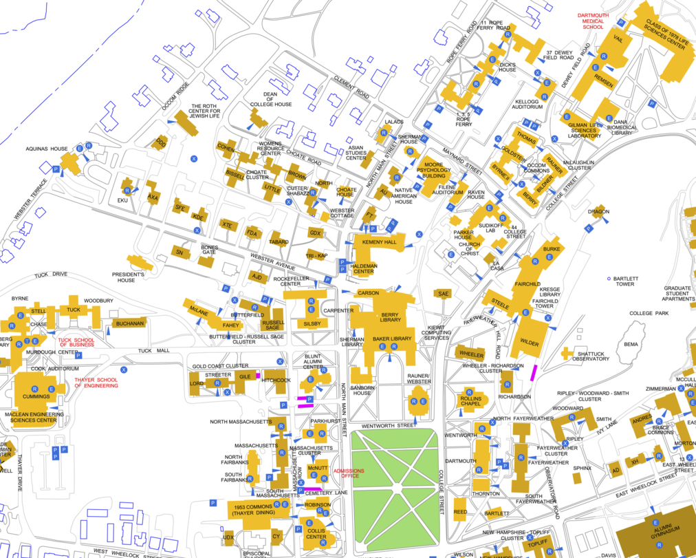
Draw the map background. The image file is dartmouth_map.png. Use the
load_imageanddraw_imagefunctions to load and display the map image. You should load the image only once; it’s a slow operation.Notice that the image is bigger than the default size for the graphics window. It’s 1012 pixels wide and 811 pixels high, so give these values as the third and fourth parameters when you call
start_graphics.Draw the graph. You have the dictionary containing information about the graph’s vertices. Each
Vertexobject has information that allows you to get x- and y-coordinates for the vertex, and it also has a list of references toVertexobjects for all adjacent vertices. You can loop over all items in the dictionary using the approach described in the notes. In addition to drawing the vertices, you should draw the edges connecting the vertices. Because the graph is undirected, each edge will appear in two adjacency lists. It’s fine to draw each edge twice.In order to draw vertices and edges, you should define methods in the
Vertexclass to do so. I have one method that draws a vertex in a color given by parameters for r, g, and b. I have one method that takes as parameters a reference to anotherVertexobject and r, g, b, and it draws an edge between theVertexthat the method is called on (i.e.,self) and the other vertex, in the color given by r, g, b. And I have one method that takes r, g, b, and draws all the edges between the vertex and all the vertices in its adjacency list, in the color given by r, g, b. I also defined constants in the vertex.py file for the radius of each vertex and the width of each edge.Allow the user to select a starting vertex for the search. As the user moves the mouse around after pressing and releasing the mouse button on a starting vertex, if the mouse is on another vertex and the button is not pressed, use this other vertex as the goal. You can call the mouse location as “on” another vertex if it’s within the smallest square that surrounds the vertex. In other words, the mouse doesn’t have to be in the circle for the vertex, but just in the smallest surrounding square; that makes the test for inclusion really simple. (Hint: Write a method in the
Vertexclass that takes as parameters x- and y-coordinates and returns a boolean indicating whether this location is within the smallest surrounding square for this vertex.)The best way I can think of doing this is, each time through your main graphics loop, check every vertex in the dictionary to see whether the mouse is on it. If you need to, you can store references to the start vertex and the goal vertex in global variables. (I didn’t need globals for them, however.) For debugging purposes, draw these two vertices in red so that you can easily see them.
Fully test and debug displaying the graph and selecting the start and goal vertices before moving on.
Using the start and goal vertices, call breadth-first search. (Write your breadth-first search function, as discussed in the next section, before coming back to this part.) The result should be a list of vertices connecting the start and goal. Draw red edges between vertices on this path to show the path from the start to the goal. An example path is shown in red on the screenshot at the top of this page. If you have both a start vertex and a goal vertex, you can call your breadth-first search function each time through the main graphics loop; it should be fast enough to allow new paths to be computed as the user moves the mouse over new locations for the goal vertex.
Breadth-first search on the graph with backchaining
Write the breadth-first search algorithm as a function in a separate file, bfs.py. map_plot.py can import this function. The breadth-first search function should take as parameters references to the start and goal vertices, and it should return a path of vertices connecting them. Represent the path by a Python list of references to Vertex objects for all vertices on the path.
Use the version of breadth-first search described in the chapter on graphs from the lecture notes. Since you need to identify all the vertices on the path between the start and the goal, you will need to keep track of backpointers and backchain to construct the path once the search has found the goal.
How to maintain the queue for the frontier
Recall that you need to maintain a queue for the frontier of your breadth-first search: the vertices that have been reached from the start vertex but have not yet been explored from. The queue needs to be first-in, first-out.
You could use a Python list for the queue. Let’s call the list q. You would insert an item, say x, by calling q.append(x), and you would remove an item by writing del q[0]. The problem is that each time you remove an item from the queue, all other items have to shift to the next lower index, which takes time linear in the size of the queue. That’s not good. We want it to take constant time to insert an item into the queue and to remove an item from the queue.
The Python collections module provides a class named deque that works as a queue with constant-time operations. In fact, it’s implemented internally with a linked list! A deque is a “double-ended queue”: you can insert into and remove from either end. You’ll use a deque as a regular queue, however. To insert, call the append method, just as you would on a Python list. To remove, call the popleft method; it takes no parameters and it removes the item in the queue that has been there the longest, returning this item. The len function returns how many items are in the queue. Example:
from collections import deque
q = deque()
q.append("Iowa")
q.append("Ohio")
print(len(q))
print(q.popleft())
print(len(q))
q.append("Idaho")
print(q.popleft())
print(q.popleft())
print(q.popleft())
As you can see, you should make sure not to call popleft when the queue is empty.
How to keep track of backpointers
You can keep track of backpointers in one of two ways. One way is to add an instance variable for a backpointer in each Vertex object. You’ll have to initialize all the backpointer instance variables for all the vertices to None upon starting each breadth-first search. The other is to make a dictionary whose keys are references to Vertex objects and whose values are also references to Vertex objects. In particular, the value for a particular key is its backpointer. For the start vertex, its value should be None, since it has no backpointer but is on the path. For the dictionary approach, initializing at the start of a breadth-first search is easy: just make an empty dictionary.
I implemented both ways, and I decided to stick with the dictionary approach. But either way is fine.
How to determine whether a vertex has been visited
Breadth-first search needs to determine whether a vertex already has been visited, because if it has, then it should not be inserted again into the queue for the frontier. One way would be to maintain a boolean in each Vertex object that tells you whether the vertex has been visited. But you’d have to initialize the boolean values for all vertices (other than the start vertex) to False each time you start a breadth-first search.
There’s an easier way. A vertex has been visited if and only if it has a backpointer. If you store backpointers in a dictionary, then to determine whether a vertex has been visited, you just need to determine whether a reference to its Vertex object appears in the dictionary. Remember that you can use the boolean in operator to determine whether an item is present in a dictionary.
Grading criteria
Checkpoint: 5 points. 3 of the 5 points are for correct behavior, and the remaining 2 points are for implementation and style.
The remaining 35 points are for the final version.
Correctness: 28 points
- Program correctly reads in the file and builds the graph: 6 points (the checkpoint also tests this behavior)
- Breadth-first search algorithm finds the goal, with minimum number of edges in paths: 10 points
- Backchaining implemented correctly: 4 points
- Graph drawing is done correctly and reasonably efficiently: 2 points
- Start and goal vertex selection works correctly: 2 points
- Drawing the path from the start vertex to the goal vertex works correctly: 2 points
- Good selection of test runs for screenshots to demonstrate a working program: 2 points
Style: 7 points
- Clear design and organization: 4 points
- Good variable names, function names, and comments: 2 points
- Correct use of instance variables: 1 point
Extra credit ideas
As usual, I encourage you to be creative in coming up with ideas for extra credit. Here are some that I thought of.
Displaying vertex names: 5 points. I demonstrated this option in class, and it appears in the screenshot above. When you display the start and goal vertices of a path, display their names, which you have in the
Vertexobjects.Add vertices to the map: 5–10 points, depending on how many you add and the quality of your work. Make sure to submit an updated dartmouth_graph.txt file if you do this option. Maybe we’ll make your file the default file we give out next time.
Animate breadth-first search: 15 points. Animate the breadth-first search process, so that we can see the breadth-first search unfold. Draw the start vertex in one color, the goal vertex in another color, and draw vertices that have been visited and searched from (that is, are no longer on the frontier) in another color, and vertices in the frontier on yet another color.
Breadcrumb search: 20 points. When searching from a specific start vertex for a specific goal vertex, the breadth-first search tree can get rather bushy. One way to cut down on the bushiness is to run two breadth-first searches simultaneously, one from the start vertex and one from the goal vertex. Each search leaves “breadcrumbs” at the vertices it has visited, and whenever a search from one of the two vertices finds a breadcrumb from the other search, it can complete a path.
What to turn in
Turn in screenshots of your program showing different paths to the goal, as well as showing the entire graph, with both vertices and edges drawn on the graph.
Also submit all source code. If you make any changes to the dartmouth_graph.txt file (say, to add more vertices for extra credit), submit the altered file as well.
Honor Code
The consequences of violating the Honor Code can be severe. Please always keep in mind the word and spirit of the Honor Code.