CS34/134 Project Report
Multi-class Object Categorization in Images
Lu He Tuobin
Wang
lu.he@dartmouth.edu tuobin.wang@dartmouth.edu
Advisor: Lorenzo Torresani
Computer Science Department
Dartmouth College
Abstract:
Object categorization is a very interesting topic
in the fields of Computer Vision and Machine Learning. Recently, the
technique of modeling the appearance of object by its distribution of
visual words has been proved successful. Our project aims to build an
image categorization and recognition system. The scenario of our system
is to load an image from the file system and user-interactively select a region from the image. Our
system can recognize the object in the selected region and output the
object name.
Introduction:
Object categorization problem is challenging
because the appearance of objects may be different due to changes of
location, illumination, pose, size and viewpoint. One type of approach
is based on the spatial arrangement of image, which use object
fragments and its spatial arrangement to represent images. Some of this
kind of model has been proved powerful, such as fragment-based models
[2, 3]. However, they can not handle variations and deformation of
objects. Moreover, they perform poorly on recognition of grass, sky and
water, which are shape-less objects. The approach applied in our
project is a kind of appearance-based method. Appearance-based methods
work well on both shape-free objects, such as sky, grass and trees, and
high-structured objects like car, face and etc.
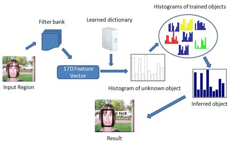
Workflow:
In our project, we implemented the algorithm published in [1]. The
workflow of our project is in the following figure:
Filter bank:
In our project, each training image is changed
into CIE L, a, b color model, and then is convolved with 17
filter-banks to generate features. The filter-banks are made of 3
Gaussians, 4 Laplacian of Gaussians (LoG) and 4 first order derivatives
of Gaussians. While the three Gaussian kernels are applied to each CIE
L, a, b channel, each with three different value σ = 1, 2, 4, the
four LoGs are applied to the L channel only, each with
four different value σ = 1,2,4,8, and the four derivative of
Gaussians kernels were divided into two x- and y- aligned set, each
with two different value σ = 2, 4. Then, we get each pixel in the
image associated with 17-dimensional feature vector.
Learn dictionary:
There are several steps to learn a final
dictionary from the training data (see the following figure).
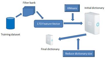
Initial Visual
Dictionary:
After image preprocessing step, each pixel in
every training image can be represented by a 17-dimensional feature
vector. We group these features together and run the unsupervised
k-means clustering algorithm with a large size of centroid number K
using the Euclidean distance. The generated K clustering centroids form
our initial visual dictionary.
Build Histogram on Dictionary:
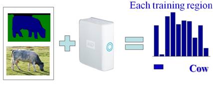
In the dataset we used, each image (left lower
image) is associated with a ground truth image (left upper image).
Labeling has been achieved for all the training images by a simple,
interactive “paint” interface. Same colors correspond to
same object classes (In our example shows above, blue color represents
cow and green color represents grass).
For each training region (only contains one single object), we want to build its histogram over the existing dictionary. Before doing this, we need to obtain the features of each training region, which can be done by extracting the positions of pixels with a specific color in the ground truth image and using these positions of pixels to get the corresponding features of each training region in the real image.
For each training region, we use statistical method to compute the corresponding histogram by simply count features that drop in each visual word. We say feature i drop in visual word j is the Euclidean distance between feature i and visual word j is smaller than the distances to all other visual words. (A histogram sample shows above).
Reduce visual
dictionary size:
We can build histograms for each training region
over the initial visual dictionary obtained from previous steps. Then,
we model the set of histograms for each class c using a Gaussian
distribution:
![]()
We define the prior probability as:
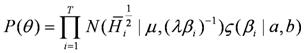
Our model is to maximizing the distribution over all the histograms given the ground truth label:
![]()
However, when
maximizing this probability, we will end up with all bins merge
together to one bin, since all histograms for any object will be
identical.
So, consider this in a different view, by applying Bayes’ rule,
what we want is to maximize:
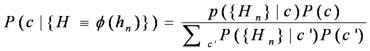
For this equation, the denominator is to penalize mappings which reduce discriminability. And, the numerator favours mappings which lead to small intra-class variance.
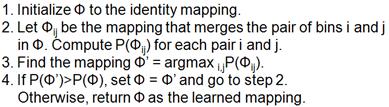
Algorithm for maximizing:
Experiment and Analysis:
We used the pixel-wise labelled image database v1
from Microsoft
Research Group, and tested our system in five objects (building,
car, face, grass and cow) by using k-nearest neighbor algorithm with k
= 1, 3, and 5. The results are in the following:
Average Trained histogram for each class:
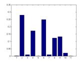
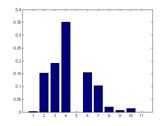
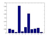
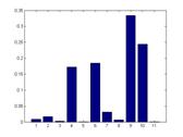
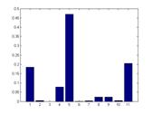
From left to right: Building, Car, Cow, Face and Grass.
Due to the large differences between different histograms above, we
confirm that our model is disciminative. On the other side, the size of
our final dictionary is 11, so our model is also compact.
Accuracy:
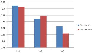
Although we reduced the dictionary size from 50 to
11, the performance does not change too much. And, one thing needs to
mention here is the result of a bigger k in kNN performs worse than a
smaller k. Our analysis is that, on the consideration of running time,
complexity and memory, we only trained a small size of data. There are
not enough trainging samples for some objects.
Confusion Matrix:
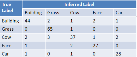
Dictionary size = 11, k = 1.
This is the confusion matrix by using kNN with k = 1 and the size of
dictionary is 11. We test 50 building, 66 grass, 45 cow, 30 face and 30
car cases. We obtained at least 82.2% accuracy of infering the true
label for each object.
GUI:
The following figure is the simple interface for
our project.
Load an image:
Select a region:

Output the result:
Reference: