Object Recognition and Tracking in Video Sequences

Abstract:

Seeing is believing, says the proverb. Though, of all our senses, the eyes are the most easily deceived, we believe them in preference to any other evidence.
[1848 J. C. & A. W. Hare Guesses at Truth (ed. 2) 2nd Ser. 497]

Object recognition in computer vision is the task of finding a given object in an image or video sequence. Object recognition is one of the hardest challenges for computer vision systems today. Humans find this task extremely trivial and can recognize objects even if they are rotated, translated, scaled or partially obstructed from view. Many approaches have been applied to object recognition in single still images or still images of the object taken from different perspectives and in different poses. We propose a supervised learning technique to extend object recognition to video sequences. The task is to be able to recognize the object and be able to track it in a video sequence. Some of the challenges posed by this particular task include recognizing the object when looking at it from a different perspective and pose, recognizing the object when it is partially occluded and tracking the object while it is in motion.

Introduction:

Humans find object recognition an easy task because they can look at the different views of the object and build up a representation of it. Object recognition is a hard problem for computer vision systems because given a single still image it is very difficult to retrieve the 3 dimensional structure of the object. For this very reason, research has moved in the direction of looking at multiple images depicting many views and poses of the same object to be able to build a better and more complete representation of the object [1], [2]. David Lowe pioneered the computer vision approach to extracting and using scale-invariant SIFT [2] features from images to perform reliable object recognition. Our approach tries to build on this by using a video sequence dataset. The video sequence consists of frames of images stitched together at a rate such that the individual images are imperceptible to the human eye and to the human eye it looks like a continuous motion. Thus in essence we are also working with single still images but the intuition is that there is more information available in video sequences rather than in single still images. It also allows us the luxury that in case we don’t have enough confidence of having seen the object in the first frame; we can look at subsequent frames to build up the confidence.

For the purpose of the project, we hung objects from a revolving mobile. The objects thus can revolve in a circular plane. Since the objects are hanging loosely and not held steadfast, they also have the freedom to rotate about their own axis and exhibit oscillatory pendulum-like motion. This unconstrained motion of the objects makes the task at hand both challenging and interesting. The video sequences were captured in greyscale using a Prosilica GC650 camera at a 640 by 480 resolution and at a frame rate of 10 frames per second. The video sequences consist of 4 objects hanging from the mobile. These objects belonged to categories similar to the ones considered in the Caltech 101 dataset [3] like cars, motorcycles, frogs etc.

Once an object is recognized, the next task is to be able to track it as it moves (displaying all the motions as explained in the previous paragraph). This task is complicated by the fact that the object while rotating on its own axis will display different poses and perspectives. Also since there are multiple objects hanging from the mobile, there is a high probability that the objects can occlude each other.

Background:

A considerable amount of previous work has addressed the task of object recognition. However, there are not many that perform the task in video sequences. Visser et al [4] talks about object recognition in videos using blob detection. Our method performs a nearest neighbor search on the image features. We use SIFT (Scale Invariant Feature Transform) [2] to extract features from the objects. Here we provide a brief overview of SIFT for the convenience of the readers. The feature extraction algorithm consists of the following steps:

• Scale-space extrema detection:
  In scale-space extrema detection the interest points called the keypoints are identified. For this image is convolved with Gaussian filters and the difference of successive Gaussian-blurred images are taken. Keypoints are then taken as maxima or minima of the difference of Gaussians.
• Keypoint localization:
  There are many keypoints obtained from step 1 of which some are unstable. These can be eliminated by performing a detailed fit to the nearby data. This is achieved using interpolation of nearby data for accurate position. Then discarding low contrast key-points and eliminating edge responses.
• Orientation assignment:
  Each keypoint is assigned one or more orientations based on image gradient directions.
• Finding the keypoint descriptor:
  The feature descriptor is computed as a set of orientation histograms on (4 x 4) pixel neighbourhoods. The orientation histograms are relative to the keypoint orientation and the orientation data comes from the Gaussian image closest in scale to the keypoint's scale. Histograms contain 8 bins each, and each descriptor contains a 4x4 array of 16 histograms around the keypoint. This leads to a SIFT feature vector with (4 x 4 x 8 = 128 elements). This vector is normalized to enhance invariance to changes in illumination.

We tried to reduce the dimensionality of the SIFT feature descriptors by performing PCA on them, but we did not get satisfactory results. Also we found that SIFT requires a minimum of 128 dimensions to represent completely the descriptor and reducing this dimensionality causes loss of important features. Hence we decided to use all the 128 dimensions in our algorithm. Instead of using a Euclidean distance metric, we use a learned Mahalanobis distance metric to compute the nearest neighbors. We learn the metric using Neighbour Components Analysis [5], a brief description of which follows. We also compute the histograms of quantized features and compare it with the histogram of the test data. For histogram comparison we compared our method with Bhattacharya co-efficient [6], diffusion distance [7] and Jeffreys–Matusita's (JM) distance [8]. We got poor results with these methods and hence we do a bin-ratio comparison across the complete histogram.

Neighbourhood Components Analysis

k-nearest neighbour (kNN) is a simple but effective method for classification. Its superior performance is due to the fact that is uses a non-linear decision boundary and the estimation rate improves as the amount of training data increases. It suffers from 2 main problems; it must store and search the entire training data for every single test point, and the modelling issue of defining the nearest neighbour distance metric. Neighbourhood Components Analysis (NCA) tries to maximize the performance of nearest neighbour classification by learning a Mahalanobis (quadratic) distance metric, which can always be represented as a positive semi-definite matrix. This distance metric is learnt by means of a linear transformation of the input space such that in the transformed space, kNN performs well.

Denoting the transformation by matrix A, we compute the learning metric as Q = A^TA such that

Although the distance metric thus learnt gives us much better results as compared to Euclidean distance, we intuited that it would be better to apply the distance metric to a more confined region so as to get rid of outliers and random noise and/or perturbations in the data. To achieve this reduction in the image space, we initially postulated that we might be able to segment out objects based on the difference in x coordinates. Thus the idea was to use a basic edge detector such as the Canny edge detector [9] to construct the edges of the individual objects. The edges which contain SIFT features i.e. edges on which SIFT features are located or the ones in whose convex hull SIFT features are found are retained and the other edges are rejected. This allowed us to look at only important edges. Now we applied a Euclidean distance between x coordinates of points on edges and wherever there was a large difference, we considered that as the start of a new object. This approach works well only if there is very little overlap between objects and the objects are separated by large enough distances in the x direction. As this is not the case for most of our video sequences, we rejected this approach.

The tracking algorithm [10] uses incremental Principal Component Analysis (PCA) with optic flow to attain tracking of the objects. It incrementally learns a low-dimensional subspace representation, adapting online to changes in the appearance of the target object. The algorithm incorporates 2 important features: a method for correctly updating the sample mean, and a forgetting factor to ensure that older observations are less likely to influence/contribute to the model.

Approach:

Given a collection of objects in video sequences, our goal is to identify the object of interest in the frame and localize it so that the co-ordinates of the object can be given to the tracking algorithm. The following steps are involved in our object recognition algorithm.

Building visual words:

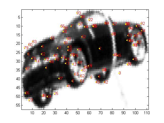
SIFT is used to extract features from object of different categories. We extract features from different views of the object as well. We quantize these features and build a code book by combining the descriptors of the objects which belong to the same category and applying k-means on these particular features. Initially we tried to take all the features from all possible categories and compute k-means on them. But k-means was unable to converge and also we were getting out of memory errors in our Matlab implementation. Thus we decided not to jumble all the features, but use category-wise features. We computed the k i.e. number of clusters, using Sturges’ formula [11].

Since this formula is used to compute the bin size for the histogram, we assume that the number of clusters from k-means denotes the number of features for the object and each bin in the histogram denotes the frequency of the number of features. So we use the same value of k for both k-means and histogram. We also perform Expectation Maximization on the clustered data obtained using k-means to obtain better clustering (Figure 1).

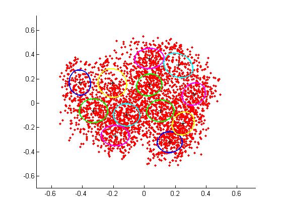
Figure 1: represents k-means applied to the car category in training dataset (Each of the ellipses represent a single cluster)

The histograms (Figure 2) of the quantized features are then computed with the bin size from (2). As mentioned earlier, each bin of the histogram denotes the number of features appearing in each cluster for each object category.

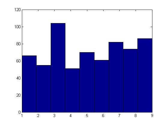
Figure 2: Histogram for the category Frog (training dataset)

We apply NCA because it is well suited to our problem and the reasons for that are listed here. Since we are working with local feature descriptors (SIFT descriptors), we can apply NCA to our data to obtain these stochastic neighbour assignments in the transformed space. Also the SIFT descriptors are 128-dimensional so it is not possible to get good distance results in the linear space with Euclidean distance. As NCA computes the distance metric which transforms the input space, we can then apply kNN to get much better distance relationships. Another advantage of using NCA is that we can restrict A to be a non-square matrix of size dxD, where d are the number of categories and D is the dimensionality of the SIFT descriptors i.e. 128.

Bounding box calculation

The test images from the video sequence consist of 4 objects and it is important to be able to segment these into separate objects. Direct computation of a distance measure on the entire image makes it very difficult to localize the position of the object of interest since there is always some random noise in the images and also some objects in particular views are unable to produce enough features. Also outlying features make it hard to compute a bounding box around the object. To resolve this problem, we initially apply a segmentation/object detection algorithm to our test images so as to obtain separate objects. The segmentation algorithm is similar to the one used in detecting prostate cancer cell in images [12]. The algorithm works on an image such as the one shown in Figure 3.

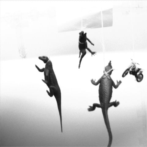
Figure 3: Original image taken from video sequence displaying 4 objects

The steps in the algorithm are as follows:

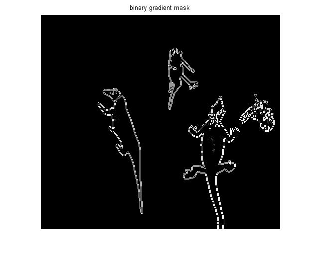
• The object to be segmented differs greatly in contrast from the background image. Changes in contrast can be detected by operators that calculate the gradient of an image. The Sobel filter is applied to obtain this binary mask which contains the segmented object (Figure 4).
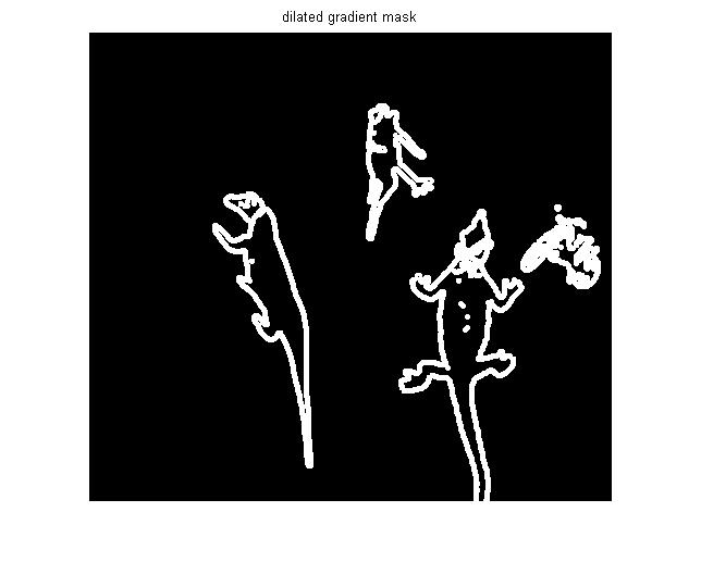
• The binary gradient mask shows lines of high contrast in the image. Compared to the original image, there are gaps in the lines surrounding the object in the gradient mask. These linear gaps disappear if the Sobel image is dilated using linear structuring elements in the vertical and horizontal directions (Figure 5).
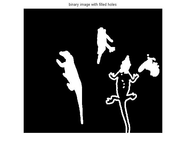
• The holes in the interior of the object are filled up (Figure 6).
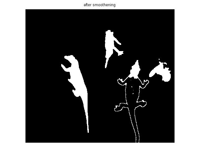
• To make the object look more natural, the object is smoothened by eroding the image twice using a diamond structuring element (Figure 7).

Figure 4: Binary Gradient Mask

Figure 5: Dilated Gradient Mask

Figure 6: Binary Image with Filled Holes

Figure 7: After Smoothening the Image

This algorithm gives us objects with continuous boundaries which are crucial for the Breadth First Search (BFS) which follows. Given the object boundaries, a BFS is run. Once a point on a boundary is explored, it is entered into a closed list to keep track of visited points. Its successors are entered into the open list to track points yet to be explored. Thus starting at a point on the boundary, the search continues till it encounters a point which doesn’t have any neighbours on the boundary or all of its neighbours are in the closed list. This search process gives us the list of points on the boundary which belong to a particular object. Using this list, we compute the bounding boxes around objects. Objects with fewer points are rejected as noise. Figures 8, 9, 10 and 11 display the bounding boxes so obtained.

Figure 8: Bounding box with Frog

Figure 9: Bounding box with Lizard 1

Figure 10: Bounding box with Lizard 2

Figure 11: Bounding box with Motorcycle

We initially tried using Depth First Search (DFS) since it is better suited to this problem as at each node (point on an edge) we need to look at successors and since the object is connected, every point on it is connected to atleast one other point in a cyclical fashion. DFS would improve the performance and allow us to converge to the goal state faster. Unfortunately Matlab gave us problems with the recursion limit, crashing when the limit was increased beyond 1000 and thus we had to reject DFS. But it is our belief that DFS would work much better than BFS for this particular case. A flaw with the edge detection approach is that when objects are touching or overlapping, the boundaries get merged and we get a bounding box consisting of more than 1 object. This is a really hard case and it is not possible to apply an edge detection or image segmentation approach to such cases. But even in such cases, the algorithm is able to localize the object to a smaller space as compared to the entire image. Also since we use multiple frames to build up our confidence, this problem gets resolved over the course of successive frames.

Experimental Results:

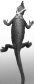
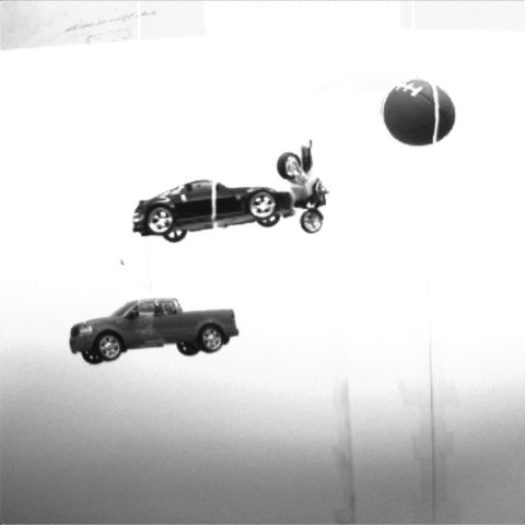
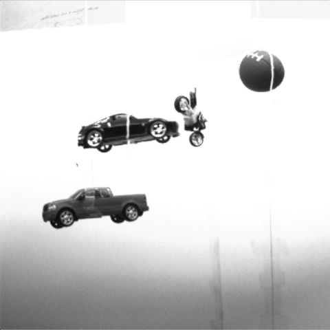
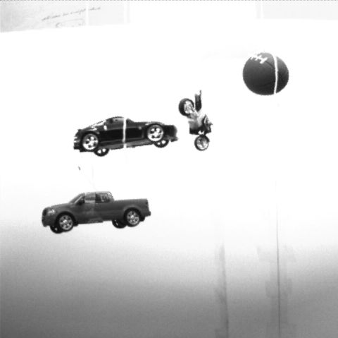
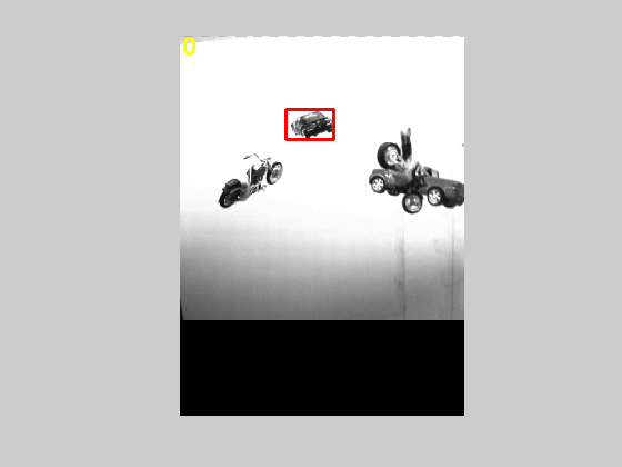
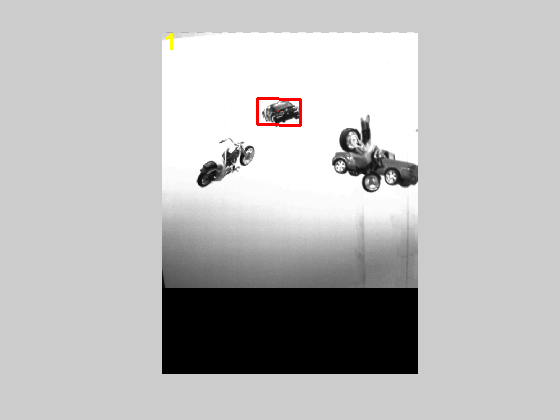
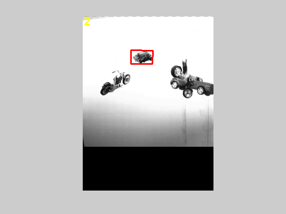
Our training dataset consists of objects from ten different categories namely motorcycles (two kinds), cars, trucks, frogs, lizards, dinosaurs, amphibians, balls and rugby balls. We have 73 images captured from different poses for the above categories and features are extracted from all of these. The objects with symmetric views had fewer images in the training set as compared to the ones with asymmetric views. Also the objects are not placed on the mobile during the training phase. We tested our algorithm on 26 video sequences with the objects on the mobile. Each video consisted of four randomly picked objects hung from the mobile. Since the objects are picked randomly, there is also a chance that objects from the same category can be on the mobile at the same time. In such a case, we consider recognition of any of the objects from the same category as a successful match. The input to the algorithm is the video sequence in which we are trying to locate an object from a specific category and the category we are interested in looking for. The frames of the video sequence are of the type shown in Figures 12-14. The objects obtained by applying the bounding boxes method to Figure 12 are shown in Figures 15-17. It is clear that the second and third objects overlapped and thus the edge detection algorithm couldn't separate them. But taking the successive frames, we are able to get separate objects thereby confirming our hypothesis that it is beneficial to look at multiple frames and not just still images. As a quantitative measure, for the 26 video sequences that we have, we obtain accurate recognition for 21 videos using multiple frames giving us a success rate of 80.77% whereas if we use single stills we get an accuracy of only 57.69%. This is displayed in Table 1. The bounding boxes obtained from the successive frame are shown in Figures 18-21.

Accuracy Measure

Multiple-frame: 			80.77%

Single still: 				57.69%

Figure 12: Test Image (Frame 1)

Figure 13: Test Image (Frame 2)

Figure 14: Test Image (Frame 3)

Figures 15, 16 and 17: Bounding boxes from frame 1

Figures 18,19, 20 and 21: Bounding boxes from frame 3

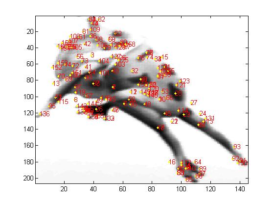
We computed the SIFT descriptors for each of the images obtained using the bounding box method explained in the Approach section. We quantize these descriptors and cluster them around the centroids we obtained by running the k-means and EM algorithms on the training dataset. This allows us to model the test data according to the distribution of the training dataset and thus provides us with a better comparison scenario (Figures 22 and 23).

Figure 22: SIFT feature descriptors from car

Figure 23: SIFT feature descriptors from frog

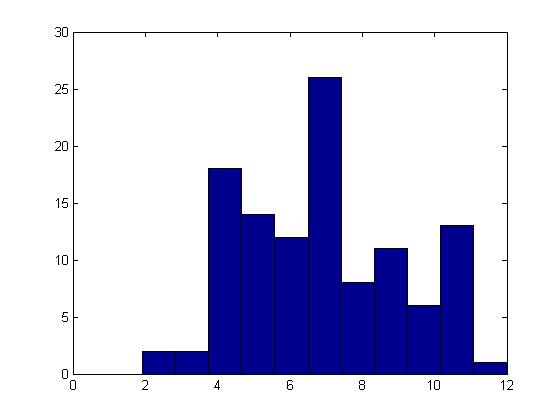
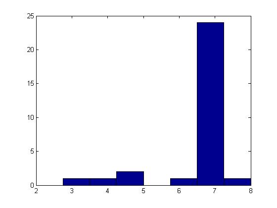
We then compute the histogram for the quantized descriptors and compare the histograms of the training and the test data by computing the bin ratio across the histograms. The histogram for the category Car from the training dataset is displayed in Figure 24 and the test set histograms for Car and Rugby Ball are displayed in Figures 25 and 26.

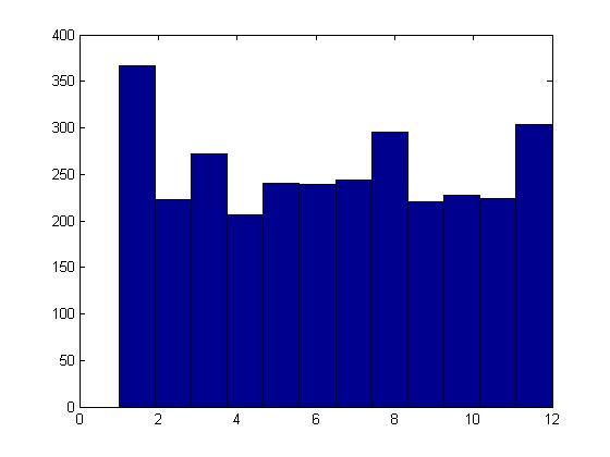
Figure 24: Histogram of car (training)

Figure 25: Histogram of car (test)

Figure 26: Histogram of rugby ball (test)

Using the learned Mahalanobis distance metric A, we compute the Mahalanobis distance between the training and the test data set using (1). The code for the implementation of the NCA algorithm was taken from the DistLearnKit link [13].The image with the best results from the histogram comparison step and distance computation step is picked as a candidate for tracking. We perform similar computations for about two-three successive frames to build confidence for our result. The intuitive idea behind this concept is that in case the object is occluded in the first frame, we may not get good results. Perhaps the object moved during the subsequent frames and hence there is a possibility of finding the object in successive frames. Once the object is found, we have the bounding box co-ordinates of the object and we provide this to the tracking algorithm. The tracking algorithm uses incremental PCA with optic flow to achieve tracking. It performs very well as long as the object is not occluded for a long period of time or there is no instantaneous change in the direction of motion of the object. A few frames depicting the tracking algorithm are shown in Figures 27-29. We propose an idea to make the algorithm more robust as part of the future work in the Conclusion section.

Figure 27: Frame 1

Figure 28: Frame 2

Figure 29: Frame 3

Figure 30 displays the Confusion Matrix of our test dataset. For categories such as Car, Lizard, Rugby Ball and Motorcycle2 we were able to obtain >80% accuracy and there were only a few False Negatives. For some of the other categories, the accuracy ratio is lower since they got misclassified as similar categories. This is the case with categories such as Motorcycle1 which gets confused often as Motorcycle2 and Frog which gets confused with Lizard and Amphibians. For some categories, we faced the problem that the objects were large and would fall over so we had to attach them with thick tape which actually resulted in addition of noise. This gave us poor results for categories such as Dinosaur and Amphibians. On an average, we were able to get a performance accuracy of 70.3% which is better than chance but we propose a few advances which would allow us to increase our performance accuracy.

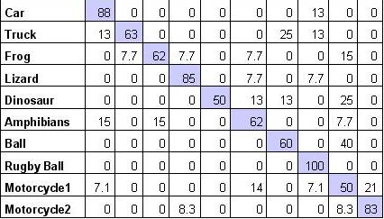
Figure 30: Confusion Matrix; Rows are ground truth and columns are model results (Performance Average = 70.3%)

Conclusion:

The task of recognizing objects was accomplished using the outlined method. We achieved results which are statistically significant (70.3%) as seen from the confusion matrix. We are thus able to track the objects across multiple frames for the video sequences. For some of the categories, we were unable to obtain good results due to similarity between categories. We propose that using more training data might help in resolving this issue. One of the interesting and important aspects of our dataset is that every test data can be used for training. Thus starting with only a few training images of the categories, we can train the algorithm iteratively as new frames are considered. Thus if the algorithm gets a particular recognition task incorrect, we can tell it in a supervised fashion that this is a false negative and that particular frame can be added to the training dataset thus incrementally building up the training dataset. Another problem we mentioned in the Experimental Results section was that we used a thick twine and non-transparent tape to hang some of the larger objects which resulted in addition of random noise. We hope to overcome this problem using thinner strings like fishing pole strings which will not be noticeable in comparison to the object. Also our camera lens was a bit faulty as can be seen from most of the images. There is a significant contrast change in the upper and lower parts of the image. We think this too might have led to some addition of noise. Using a different camera would help resolve this issue.

As part of the future work, we would like to add more categories to the training data and also use a changing background instead of a plain background. This is a difficult task since now we would have to contend with not only multiple objects on the mobile but also background clutter. In respect to the tracking algorithm, it can be made robust enough to handle instantaneous changes in direction of motion. Also in the case where the object is no longer in the bounding box, the tracking algorithm needs to apply the recognition algorithm iteratively to localize the object again. This would be a significantly challenging task since presently the tracking algorithm cannot understand that it has lost the object. It continues to place the bounding box in positions which have the highest probability of getting the object given the position of the object in the previous frame. This basic conditional probability assumption doesn't hold true for cases where the object gets completely occluded or changes its direction of motion.

Acknowledgements:

We would like to acknowledge Prof. Torresani, Prof. Granger, Prof. Felch and Wei Pan for their valuable suggestions and guidance throughout the implementation of this project.

References:

• C. Schmid, R. Mohr. Local Greyvalue Invariants for Image Retrieval. In IEEE Transactions on Pattern Analysis and Machine Intelligence, 1997.
• D. Lowe. Distinctive Image Features from Scale-Invariant Keypoints. In International Journal of Computer Vision, 2004.
• Caltech 101 http://www.vision.caltech.edu/Image_Datasets/Caltech101/
• R. Visser, N. Sebe, E. Bakker. Object Recognition for Video Retrieval
• J. Goldberger, S. Roweis, G. Hinton, R. Salakhutdinov. Neighbourhood Components Analysis. in Advances in Neural Information Processing Systems, 2005.
• M. Sohail Khalid, M. Bilal Malik. Biased Nature of Bhattacharyya Coefficient in Correlation of Gray-Scale Objects.
• H. Ling, K. Okada. Diffusion Distance for Histogram Comparison. In Proc. IEEE. Conf. on Computer Vision and Pattern Recognition, 2006.
• R. A. Schowengerdt. Techniques for Image Processing and Classification in Remote Sensing. Academia Press, INC, 1983.
• Canny, J. A Computational Approach To Edge Detection. In IEEE Trans. Pattern Analysis and Machine Intelligence, 8:679-714, 1986.
• D. A. Ross, J. Lim, R. Lin, M. Yang. Incremental Learning for Robust Visual Tracking. In International Journal of Computer Vision (IJCV), 2008.
• Sturges, H. A. The choice of a class interval. In J. American Statistical Association: 65–66, 1926.
• Image Processing Toolbox- Detecting a Cell Using Image Segmentation Demo
  http://www.mathworks.com/products/image/demos.html?file=/products/demos/shipping/images/ipexcell.html
• DistLearnKit: Matlab Toolkit for Distance Metric Learning http://www.cs.cmu.edu/~liuy/distlearn.htm