This forced us to do some pre-processing of the data that would help alleviate this issue.
Current inrush is a phenomenon that occurs when certain devices are switched on. A spike in current during the switching on of an electronic device happens because components in these devices (i.e. heating elements, transformers, motors) have very low impedance until they reach their normal operational conditions. An incandescent light bulb, for example, has very low impedance when the tungsten element is cold but once it is switched on, the element heats up in a matter of milliseconds and the impedance increases dramatically. The way in which the impedance settles to its steady state is unique to the light, transformer or motor and can provide a fingerprint for identifying the device.
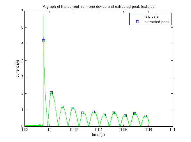
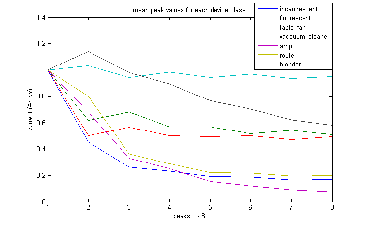
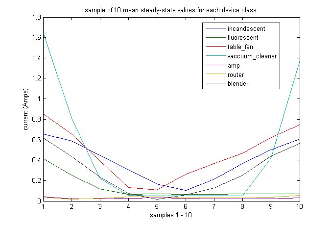
In our project, the goal was to classify different inrush current decay curves so as to determine the type of device. We approached the problem from an experimental point of view, looking at different aspects of the raw data (the current curves) until we were able to identify some useful features in the data. We obtained the decay curves by extracting the peaks in the current curves (see the section on "Peak Extraction"). Noting that these features alone were inadequate to effectively classify the 173 test examples our seven classes of electrical devices, we added a new set of features (the steady-state samples) that allowed us to see the shapes of the stead-state current curves. We then used largest margin nearest neighbor (LMNN) to classify the devices based on a learned distance metric, as opposed to a simple Euclidean distance metric. In the end, with these new additions to our methodology we were able to accomplish our goals with an exciting degree of accuracy.
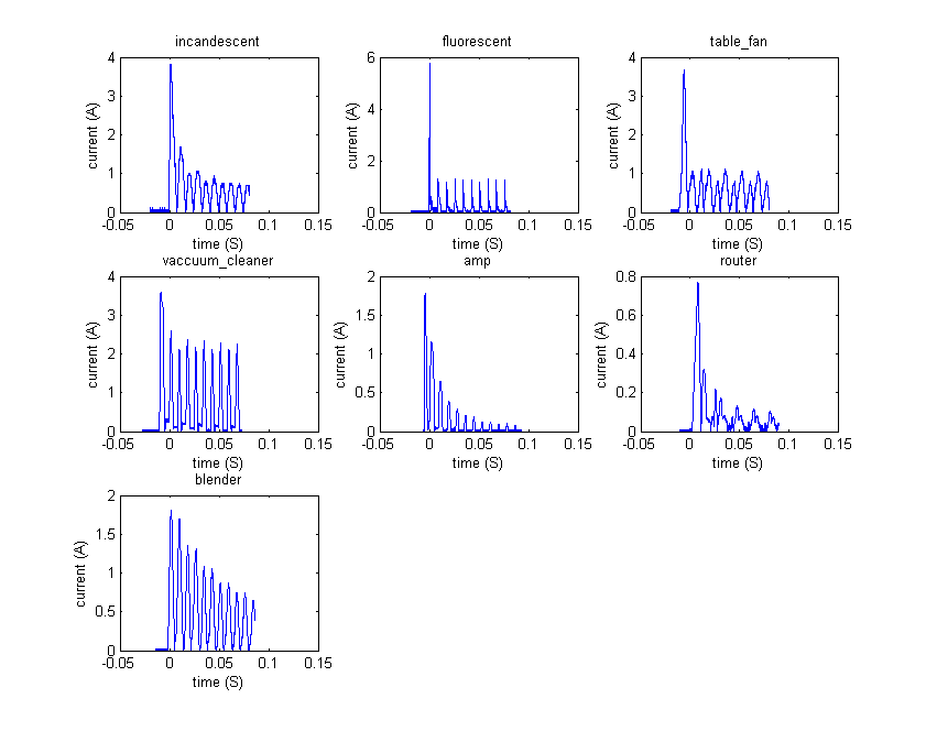
We recorded data from 7 different types of devices:
The main difficulty that arises has to do with the effect that AC (alternating current) has on the data we collect from the oscilloscope. The inrush peak for a device like a lightbulb, is proportional to the amount of instantaneous current available when switched on. In the case of alternating current, the magnitude of current that is available from the socket is sinusoidal with a frequency of 60Hz. Therefore, 120 times a second, there will be times of peak current and zero current, each 90 degrees phase shifted from each other. When the device is turned on at the peaks, the inrush current is greatest. When the device is turned on at times of zero current, or "zero crossings," the inrush is barely measureable.
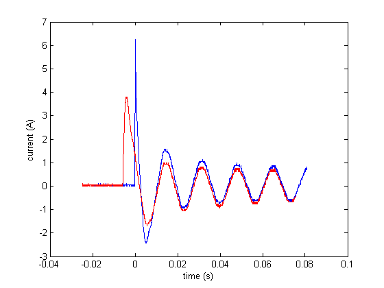
This results in two things: (1) there is a different amount of time between the initial inrush peak and the second peak (for an example, see the image above). And (2) the initial peaks can have varying magnitudes (see above image). We felt that both of these results would make extracting meaningful feutures via regression problematic. Instead we have devised a two-fold feature extraction scheme, which is outlined in the "Peak Extraction" and "Steady-state sampling" sections below.
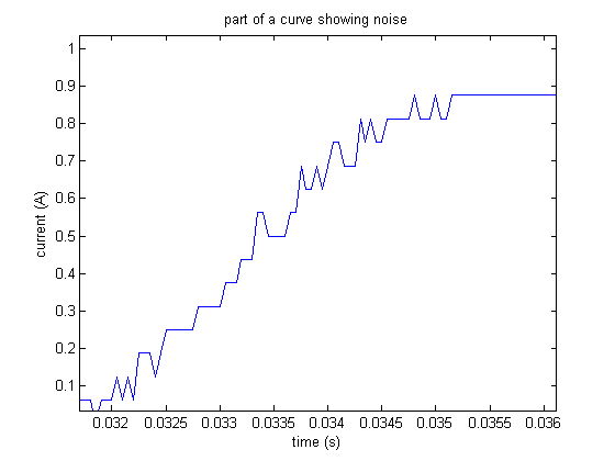
Another problem with the data that affected our feature extraction algorithm was noise. Here is a section of a curve showing the amount of noise:
This forced us to do some pre-processing of the data that would help alleviate this issue.
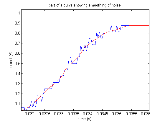
First, to remove some of the noise from the raw data, we employed a MATLAB smoothing function, smooth(V, 15, 'lowess'), where V was the vector containing the Current values for some example curve. This smoothing function employed local regression using weighted linear least squares and a 1st degree polynomial model with a span of 15 points. Here we see how well it smoothed the noisy data shown in image above (the red line is the result of the smoothing function):
After smoothing, we took the absolute value of the current values in order to make the process of finding peaks easier -- instead of searching for local maxima and local minima, we only need to search for local maxima.
Less Successful Method
For each example curve:
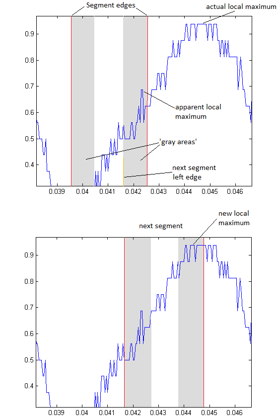
More Successful Method
This method behaves exactly the same as the above method, except that we search backwards (from a point where the peaks are consistently spaced).

Largest margin nearest neighbor (LMNN) learns a Mahanalobis distance metric for kNN. The goal is a metric where the “k-nearest neighbors always belong to the same class while examples from different classes are separated by a large margin”[1].

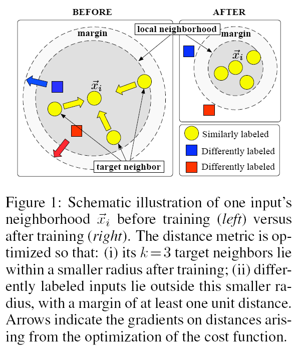 from [1].
We ran a 'rough ablative analysis' to see the effects of our choice of features. It was not a true ablative analysis because we did not remove each feature one-by-one. Instead we looked at our classification results after removing one of the sets of features that were described in the section above. For these tests k = 3.
We began with the normal case, including all 19 features (peak features, time feature, and steady-state sample features).
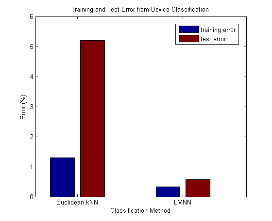
Here we immediately see the impact of the improved distance metric learned through LMNN. We had a test error of 5.2% with kNN using Euclidean distance; but when we learned an optimal distance metric with LMNN, we ended up with a test error of only 0.58%. Furthermore it only took 11.33 seconds to train this model. We have both accuracy and speed here.
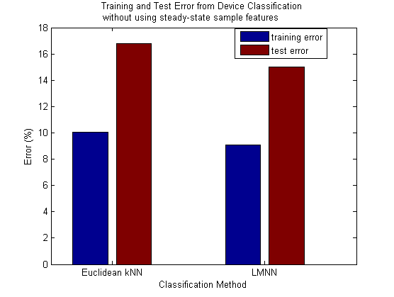
Now we will look at what happens when we remove the 8 peak features -- we're classifying with 11 features: the 10 steady-state sample features and the 1 time feature.
This gives us some strange results in the case of normal kNN. The training error is actually higher than the test error. We get a good test error here for normal kNN with Euclidean distance (around 1.5%). It actually beats the LMNN test error here, which is quite high compared to the previous test. Another thing to note here is that training this time took almost 10 times as long as the previous example. It took just under 104 seconds. One might expect that reducing the number of features would reduce the training time, but here with some of the features withheld LMNN needs to work much longer to find an optimal distance metric. This certainly shows the importance of the peak features as a group.
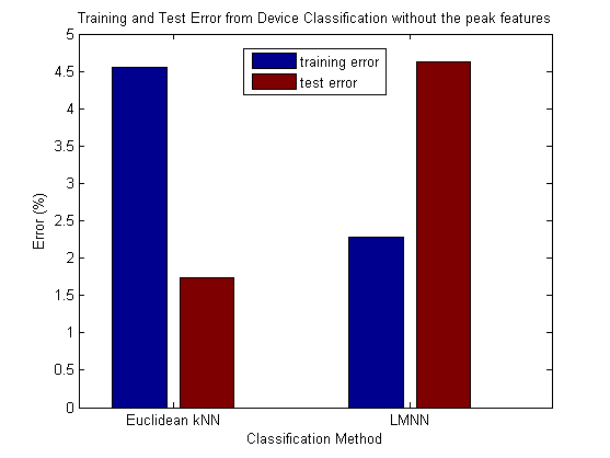
Last we will explore the effect of withholding the steady-state sample set. Now we are using 9 features to classify: the 8 peak features and the 1 time feature.
Here the LMNN reduces the amount of error slightly from the error that Euclidean kNN got. However, both errors are very high -- over 16% for Euclidean kNN and around 15% for LMNN. This very clearly identifies the steady-state sample features as the most important set of features for our classification system. For LMNN we get a drop of around 14.5% when we add the steady-state sample features back into our full set of features. The training time here was 34.82 seconds, which is still significantly higher than the training time with the full set of features (11.33 seconds). This again tells us that the features used here are insufficient for LMNN and it therefore take a longer time trying to find an optimal metric, because an optimal metric is harder to come by with this set of features.
Removing the time feature from the set had no effect whatsoever on the training or test error for either Euclidean kNN or LMNN. We could safely remove the attribute without any repercussions.
Lastly we will look at all of the LMNN errors together:
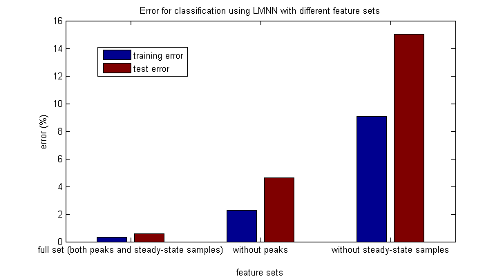
It becomes quite clear that our full set of features (minus the time feature) is the best set of features to use for classification with LMNN. As we remove features (moving right along the chart), we see that our model is underfitting. The reduced set of features is inadequate for describing the complexity of the problem. On the other hand, the full set of features combined with the new distance metric learned through LMNN allows for a high degree of accuracy while maintaining an impressive training speed.