CS 34/134 Machine Learning & Stat Analysis
Spring 2009
Learning to Classify Telemarketing Phone Numbers
Yiming Qi & Zhiyuan Zhang
Motivation
Almost every person has experienced the annoyance of telemarketing phone calls, which occur at inopportune times and repeat with high frequency. While persons can sign themselves up on the national Do Not Call Registry, which is a list of phone owners that telemarketers cannot legally call, there are several disadvantages to doing so: it is bothersome to sign up, the jurisdiction of the list is limited in scope, and block all telemarketing calls uniformly even if the person wanted some calls to come through. Moreover, many telemarketers call with spoofed numbers to trick caller ID owners and avoid legal telemarketing restrictions. Therefore, it will be useful to know whether an incoming phone call is going to be a telemarketing call before picking it up. With 10 billion possible phone numbers in the US and no obvious underlying pattern of those numbers, it is difficult to differentiate telemarketing phone numbers from unidentified phone numbers which might come from friends, family, or clients. One of the authors has had extensive personal experiences with undesirable telemarketing calls, and therefore we are enthusiastic about finding a solution to tackle this real-life problem.
Goal
We will classify calls as "undesirable" (telemarketers, debt collectors, political canvassers, prank callers, and any other complained-about numbers) and "desirable" (everything else) given only the phone number.
Data
To obtain telephone numbers, we created a web crawler to html-scrape within the confines of two sites, www.callercomplaints.com and www.yellowpages.com, to obtain "bad" and "good" phone numbers from the sites respectively. Caller Complaints was completely scraped; we obtained 385,285 bad phone numbers from the site. Yellow Pages was not completely scraped; because the site is meant for use by service seekers it provides much extraneous info in addition to telephone numbers (such as business ratings and customer reviews), so the telephone number density was much lower for the yellow pages than it was for Caller Complaints. The Yellow Pages also contains the phone number of almost every registered business and person in the United States, so we did not expect to web-crawl the entire site. We stopped the crawler for the Yellow Pages to obtain 124,971 good telephone numbers. It should be noted that we parsed are fewer numbers from the Yellow Pages than from the Caller Complaints site, but those fewer numbers took a much longer time to obtain because the telephone number density was extremely low. In addition, the web crawler crawls links in non-deterministic order, which means that our telephone numbers come from a random distribution that we assume to be independently and identically distributed.
We interpreted the data in two different froms of dimensionality, ten dimensional and three dimensional. Ten dimensional data uses each digit as a feature, and three dimensional data uses each block (commonly separated by hyphens or spaces) as a feature. Splitting the telephone numbers into ten dimensions is natural, and our motivation for splitting the number into three dimensions comes from the anecdotal observation that phone numbers sharing common blocks are geographically related.
Because we have much more bad telephone numbers than good telephone numbers, our machine learning techniques may be biased by this uneven data distribution. We therefore normalize our training data by taking even amounts of good and bad telephone numbers when we train our various techniques. The data order is also randomized, so any sequential order in the data resulting from web crawling is disregarded. This is important because we train on a subset of the data, reserving a small chunk for testing, so the data should be randomly ordered so as to create independently and identically distributed data. Therefore, we have a total of 249,942 telephone numbers, split evenly into good and bad phone numbers.
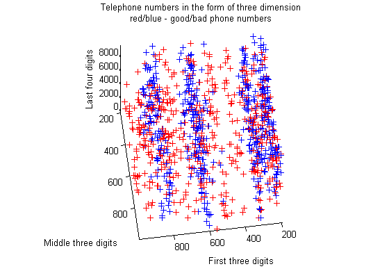
Distribution
To help visualize our data and see if we can human-learn any patterns, we created a three dimensional graph of the 500 randomly selected good telephone numbers and 500 randomly selected bad telephone numbers, interpreted as three dimensional blocks. This attempt reveals that phone numbers are tightly clustered around "century" values (a "century" value is what we call the first block of telephone numbers), and that there are several "century" values for which bad phone numbers are rare, but good phone numbers are common. We can easily perceive that the decision boundary for some of the phone numbers form parallel planes, which indicates that our data requires a non-linear decision boundary.
Methods
Decision Trees
This is our best classifier, because the parallel decision planes observed in the visualization of telephone numbers look like perfect candidates for decision-tree classification. For our decision tree (and naive Bayes classifier) we preprocess our training data by converting each ten-dimensional telephone number into a 100-dimensional vector, where each digit in the original telephone number maps to a ten-dimensional vector of zeros, except for one 1 in the nth position of the vector, where n is the digit (e.g., 9 would translate to 0000000010, and 5 would translate to 0000100000; 0 would be represented by a sequence of 9 0s and one 1.). This new feature vector is then input to a decision tree with binary decision tests and a stopping condition that stops splitting after the number of training examples assigned to a node drops below a certain fraction of (C) of the total number of nodes. This decision tree makes decisions based on the value of each digit. The reason why we expanded the input vector instead of changing the binary decision tree to an n-ary decision tree is because this new encoding of a telephone number will prove useful in Naive Bayes as well, and is simpler to implement than an n-ary tree. We created and evaluated 7 different decision trees, all of which are trained on 200,000 examples and tested on 49,942 examples, each of which has a different C, with C being .0001, .0005, .001, .005, .01, .05, or .1
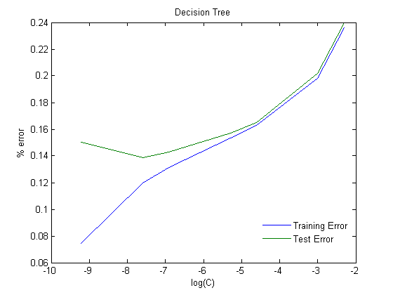
This graph shows classic underfitting on the right end, and overfitting on the left end. We picked .0005 as the best C, as it showed the least test and training error.
error on whole data set (%) |
misclassification rate for good phone numbers (%) |
misclassification rate for bad phone numbers (%) |
|
Trainng |
11.98 |
14.67 |
9.28 |
Test |
13.86 |
16.28 |
11.46 |
The decision tree classifies bad phone numbers slightly more accurately than good phone numbers, which would be worrisome were it not for the misclassification rates of the other learning algorithms. Compared to our other results, a misclassification rate of 16% on the test set's good phone numbers is outstanding.
Naive Bayes
Using a Naive Bayes classifier is a natural choice for classifying good and bad telephone numbers, as the requirements for classifying telephone numbers is similar to that of classifying emails as spam or ham - it would be best to have a soft decision boundary, with probabilistic classification decisions, and it handles high dimensionality easily. We preprocess our training data by converting each ten-dimensional telephone number into a 100-dimensional vector, where each digit in the original telephone number maps to a ten-dimensional vector of zeros, except for one 1 in the nth position of the vector, where n is the digit (e.g., 9 would translate to 0000000010, and 5 would translate to 0000100000; 0 would be represented by a sequence of 9 0s and one 1.). This new feature vector is then the input to a naive Bayes classifier with a Bernoulli distribution. We transform the training data in this unconventional way because we perceived the problem as essentially analogous to classifying a fixed-length email as spam or ham.
Using Naive Bayes on 200,000 training examples and 49,942 test examples, we obtain the following result:
error on whole data set (%) |
misclassification rate for good phone numbers (%) |
misclassification rate for bad phone numbers (%) |
|
Trainng |
25.92 |
40.71 |
11.10 |
Test |
26.18 |
41.30 |
11.18 |
Naive Bayes has similar misclassification rates on bad phone numbers as that of decistion trees, but has a very high misclassification rate for good phone numbers. This extremely high rate makes Naive Bayes essentially unusable.
k-NN
We transformed our training data (both ten-dimensional and three-dimensional) with Relevant Component Analysis to weigh relevant features more heavily before running k-nearest neighbors. We ran k-NN with both the ten-dimensional and the three-dimensional feature vector training sets.
We tested several dozen choices for k, with each test having 100,000 training examples and 100 test examples (k-NN is expensive to test, hence the small number of test examples when running k-NN over many ks in sequence).
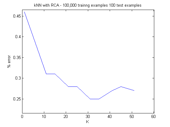
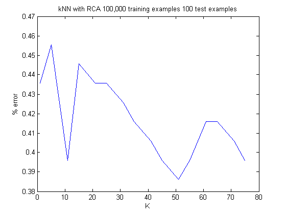
Picking the best value of k (lowest test error) for each data set, we ran k-NN on 100,000 training examples and 1,000 test examples, to arrive at a 29.77% test error for the three-dimensional data set and 29.37% test error for the ten-dimensional data set.
The minimum test error (within the range of ks we have tested) for data of both dimensions is similar, but the test error for three-dimensional data vary much more than the test error for ten-dimensional data as k increases. This indicates that reducing the dimensionality of the data by logical telephone blocks may not be a good idea, because it means that k-NN's wavering predictions show that the decision boundary is very complex, which implies that the data may be clustered arbitrarily and result in a poor training set after dimensionality reduction. The learning algorithms which we have ran after discovering this variation, namely Naive Bayes, Decision Trees, and SVM, all use ten-dimensional data in light of this observation.
The misclassification rates of k-NN on ten-dimensional and three-dimensional data are shown in the chart below.
error on whole data set (%) |
misclassification rate for good phone numbers (%) |
misclassification rate for bad phone numbers (%) |
|
10D |
29.37 |
32.39 |
26.39 |
3D |
29.77 |
43.70 |
16.31 |
Using ten-dimensional data instead of three-dimensional data causes an increase in the misclassification rate of bad phone numbers, but reduces the misclassification rate of good phone numbers. Because we value accuracy on good phone numbers more than accuracy on bad phone numbers, this reinforces our decision to use ten-dimensional data.
Without RCA weighing our features, the ten-dimensional k-NN test error was around 35%. RCA improved our test error by 6%.
SVM
As we noted before, parts of the data appeared to be separated by multiple linear boundaries (planes separating phone numbers based on century values). This motivated our decision to use a linear SVM on the training set, because these easily human-perceivable linear boundaries suggested that a higher-dimensional mapping of our data may indeed contain a linear boundary learnable by SVM. We implemented SVM with simple quadratic programming, on 1000 training examples. Because the visualization of phone numbers only contained 1000 examples and already depicted salient boundaries, we believed using 1000 examples in the training set would be sufficient to learn a decision boundary. In addition, we tweaked the number of training examples to see if we would get better results by using more or fewer examples.
| Training Examples | Test Examples | Training Error (%) | Test Error |
| 500 | 500 | 42.6 | 43.0 |
| 700 | 10000 | 45.0 | 46.7 |
| 1000 | 10000 | 39.3 | 40.5 |
As is expected, the training error and test error reduces as test examples increase. However, because our implementation of SVM is slow and we have much faster and more accurate learning algorithms, we chose to not go forward with larger training sets or tweaking more parameters.
Logistic Regression
Although we knew that the data could not be described by a linear boundary, we still ran logistic regression to see what we could learn from its results. We ran the algorithm on the ten-dimensional data set with 5,000 training examples and a learning rate determined by line sesarch. After 586 iterations, it converged to a model which produced a 40.22% training error and 40.82% test error.
The results were very poor, but because logistic regression was one of the first algorithms we ran, we were encouraged by the below-50% test error. This showed us that the commonsense assumption that telephone numbers are uniformly distributed is not true, and that there is indeed an underlying pattern to the phone numbers which we can exploit with further learning algorithms. We did not tweak the parameters of logistic regression any further because we knew it was the wrong model for our problem - logistic regressions describe a linear boundary, which our data does not have.
Neural Network
Our first attempt at solving the problem was with a multi-layered neural network. We used 10 input signals, 2 output signals, a middle layer with 10 nodes, and an learning rate of 0.5. After 10,000 training cycles on 1,000 training examples, we observed a 50% training error, which is no better than guessing. We also tried 0 nodes and 5 nodes on the middle layer, all of which prodcuced the same results. We did not experiment with neural networks any further after receiving these discouraging results.
Conclusion
Our intuition was correct: the parallel decision boundaries that we perceived from the visualization of data was easily learned by a decision tree, which produced decent classification results with the smallest misclassification rates on both good and bad telephone numbers. We were surprised that k-NN and Naive Bayes produced such a high misclassification rate for good phone numbers compared to bad ones. We speculate that this is due to the sparseness of good phone numbers - the misclassification rates seem to indicate bad phone numbers are closely spaced together, whereas good phone numbers are scattered all over the phone number space. Such a distribution would distort k-NN boundaries, and the lack of underlying pattern in good phone numbers would cause the high Naive Bayes misclassification rate.
Acknowledgements
We would like to thank Professor Torresani for his advice on learning a distance metric for k-NN, and his skepticism at our original attempts to classify the data with decision trees and Naive Bayes, which led to us changing our models and greatly improving our error rates. We would also like to thank Professors Bar-Hillel and Hertz, who shared their RCA code on the Carnegie Mellon University website.
We would like to thank our T.A., Wei Pan, for posting our milestones and project proposals on the course site.
References
Bar-Hillel, Aharon., Tomer Hertz, Noam Shental, Daphna Weinshall, Learning Distance Functions using Equivalence Relations. Proceedings of the Twentieth International Conference on Machine Learning (ICML-2003), Washington, 2003.
Bishop, Christopher M., Pattern Recognition and Machine Learning, Springer, 2006
Burges, Christopher J.C., A Tutorial on Support Vector Machines for Pattern Recgonition, Data Mining and Knowledge Discovery, 2, 121―167 (1998)
Kononenko, Igor., Machine Learning and Data Mining: Introduction to Principles and Algorithms, Horwood Publishing, 2007.