Project Milestone
Yiming Qi & Zhiyuan Zhang
May 12, 2009
Learning to Classify and Forecast Telemarketing Phone Numbers
Overview
For the milestone, we have implemented and run neural networks, k-nearest neighbors (kNN), and logistic regression on our test data. A major hurdle was the massive amount of data we obtained, which made training very time-consuming and difficult. We decided to train on several smaller subsets of our data in order to see the effects different parameters have on our models, and train on larger data sets in the future based on the results of our evaluation of the models. kNN was our most successful model, with logistic regression a close second. Our neural network did not perform so well, with results oscillating around 50% (meaning it is not better than random guessing).
Data
To obtain telephone numbers, we created a web crawler to html-scrape within the confines of two sites, www.callercomplaints.com and www.yellowpages.com, to obtain "bad" and "good" phone numbers from the sites respectively. Caller Complaints was completely scraped; we obtained 385,285 bad phone numbers from the site. Yellow Pages was not completely scraped; because the site is meant for use by service seekers it provides much extraneous info in addition to telephone numbers (such as business ratings and customer reviews), so the telephone number density was much lower for the yellow pages than it was for Caller Complaints. The Yellow Pages also contains the phone number of almost every registered business and person in the United States, so we did not expect to web-crawl the entire site. The crawler was stopped prematurely for the Yellow Pages to obtain 124,971 good telephone numbers. It should be noted that we parsed are fewer numbers from the Yellow Pages than from the Caller Complaints site, but those fewer numbers took a much longer time to obtain because the telephone number density was extremely low.
We interpreted the data in two different froms of dimensionality, ten dimensional and three dimensional. Ten dimensional data uses each digit as a feature, and three dimensional data uses each block (commonly separated by hyphens or spaces) as a feature. Splitting the telephone numbers into ten dimensions is natural, and our motivation for splitting the number into three dimensions comes from the anecdotal observation that phone numbers sharing common blocks are geographically related.
Because we have much more bad telephone numbers than good telephone numbers, our machine learning techniques may be biased by this uneven data distribution. We therefore use even amounts of good and bad telephone numbers when we train our various techniques. The data order is also randomized, so any sequential order in the data as a result of web crawling is disregarded. This is important because we train on only a subset of the data, which is the first several thousand data set values, so the data should be randomly ordered so as to create independently and identically distributed data.
Distribution
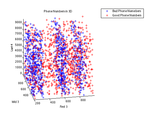
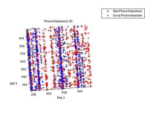
To help visualize our data and see if we can human-learn any patterns, we created a three dimensional graph of the 500 good telephone numbers and 500 bad telephone numbers, interpreted as three dimensional blocks. This preliminary attempt (see phonenum3d.fig) reveals that phone numbers are tightly clustered around "century" values (e.g., most 4xx-xxx-xxxx phone numbers have the first block close to 400, as opposed to being uniformly distributed between 400 and 500), and that there are several "century" values for which bad phone numbers are rare, but good phone numbers are common.
Classification using Neural Network
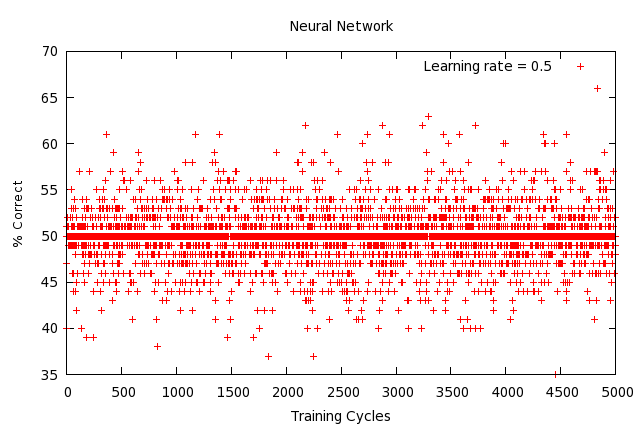
We had a copy of the neural network data structure and the back-propagation algorithm that Karn and Yiming implemented in CS44 last winter for their face identification project. We made some modifications to the code so that our phone number data can be fed into the neural network. ?Since each phone number consists of 10 digits, we first decided to test the performance of our neural network by treating each input phone number as a 10-dimension vector. We experimented with a three-layer network for training and testing: 10 input signals in the first layer, 0, 10, and 20 nodes in the middle layer, and 2 output signals in the output layer. We decided the class label as either “good” or “bad” for each training example by picking the larger probability we obtained from the two output signals of the neural network.? We trained the neural network for 10,000 training cycles on 1000 training examples (containing 500 good phone numbers, and 500 telemarketing phone numbers). We then tested our neural network on a test set containing 100 good and 100 bad phone numbers. The percentage correct turned out to be exactly 50%, which means the classification was no better than random guessing. We then tried to change the dimensionality of the input vector to 3, equivalent to xxx-xxx-xxxx. ?We repeated the training and testing process and got a similar result, as shown below. The reason that neural network did not learn so well to classify the two classes was probably because we have not provided the network with large enough training-set examples and training cycles. Right now, we are mainly interested in the performance of the neural network on a small subset of our data to see how well it learns. Our conclusion is that neural network is slow to learn and we will have to spend more time training the network before testing it.
Classification using Logistic Regression
We also experimented using the logistic regression code in matlab that we implemented for homework 1 to classify the good and bad phone numbers. Our training set consisted of 5000 phone numbers randomly selected from the whole data set. Our test set consisted of a subset of 5000 phone numbers that is disjoint from the training set. We employed the line search algorithm to compute the learning rate alpha and went through 586 iterations to have the log likelihood reach convergence. The percentage correct of the training set turns out to be 59.78%, and 59.18% for the test set. ?Logistic regression runs much faster on a larger training set than neural network, and does a better performance.
Classification using kNN
We implemented k-nearest neighbors to run on the entire data set. The algorithm simply tallies up the kth nearest (in terms of euclidean distance) neighbors and classifies the test example based on the vote of the neighbors - each neighbor has one vote and the classification is decided by which class the majority of the neighbors belong to. We ran the algorithm on two data sets, one in which a phone number is a 10-dimensional feature vector (one digit is a feature) and the other in which a phone number is a 3-dimensional feature vector. We did not run it on the entire data set, as kNN is extremely expensive to test; instead, for both sets of data, we ran kNN on 50,000 data set values. Odd-numbered values of k were attempted, from 1 to 9 inclusively, and validated by a variant of cross-validation which we call "random" validation. "Random" validation operates in the same fashion as cross-validation, except instead of testing kNN against each test example in the test set, we only test kNN against a certain number of randomly selected test examples within the test set. For the purposes of the milestone we ran 5-fold cross validation and tested kNN on 50 test examples within each test set. The results are shown below.
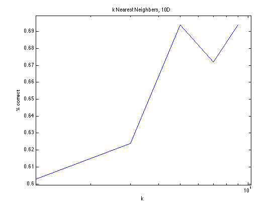
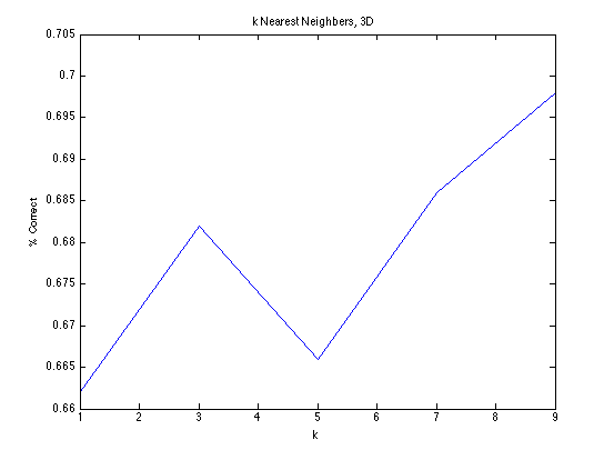
kNN displays a curious increase in correctness as k increases. We believe this may be because we are selecting k to be too small; however, the variation in k with k > 1 is not very large in absolute terms, so it is not particularly worrisome. Both ten dimensional and three dimensional data sets hover between 65% to 70% correctness, although kNN performs slightly better on three dimensional data than ten dimensional data (the highest value of percentage correct is smaller for kNN10D by one percent).
Classification using Logistic Regression
We also experimented using the logistic regression code in matlab that we implemented for homework 1 to classify the good and bad phone numbers. Our training set consisted of 5000 phone numbers randomly selected from the whole data set. Our test set consisted of a subset of 5000 phone numbers that is disjoint from the training set. We employed the line search algorithm to compute the learning rate alpha and went through 586 iterations to have the log likelihood reach convergence. The percentage correct of the training set turns out to be 59.78%, and 59.18% for the test set. Logistic regression runs much faster on a larger training set than neural network, and does a better performance.
Future
Our plan is to spend enough time training the neural network with 75% of the “bad” phone numbers (approximately 288963 phone numbers) and 75% of the “good” phone numbers (approximately 93728 phone numbers) we have crawled so far. We will use the resulting neural network to test on the remaining data we have and report a percentage correct with a few learning rates and layer sizes in our final report.
kNN and logistic regression are both good candidates for classifying telephone numbers. Because kNN is easier to evaluate and simpler to debug, we will go with kNN when proceeding with our goal for the second half of the project, which is adding in time as another dimension. We will try weighted euclidean distance with kNN, weighing time more heavily than other dimensions. We will also consider other classifiers, such as Naive Bayes and Support Vector Machines, as other possible candidates. Another possible way to increase our correctness is to consider both kNN and logistic regression as weak classifiers, and use adaptive boosting to combine the two to reduce our error.