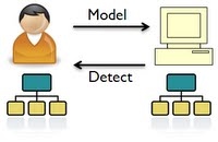
Deqing Li Project OverviewIn this project, I detect deception by learning Bayesian Networks using machine learning techniques. Specifically, human experts are simulated by BNs and then the parameters of their simulators, which are the conditional probability tables (CPTs), are learned from observations generated from the simulators assuming that we already know the structure of the simulator BN. To test the reliability of the learned model, I reason through the model and compare the answers with the experts' answer inferred from the simulator. Here, the answer of the model/simulator refers to the posterior probability distributions inferred from the corresponding BNs. To detect deception, the answers from the model are compared with the deceptive answers from the simulator. An architecture of the system is shown in Figure 1. Fig. 1 Architecture of Deception Detection by Learning Bayesian Networks Achievements
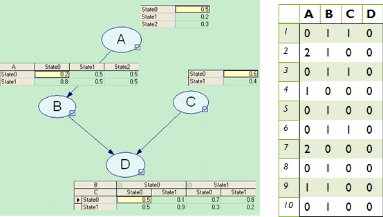
A set of training data is in the format of "r.v.(i,j) = state(i,j)" where i represents the ith sample and j represents the jth
random variable. The state of each r.v. is generated randomly according
to its CPT. To ease the process of generating data, the states of the
root nodes, which are not conditioning on any other nodes, are
generated first. Then, based on their states, generate the states of
their children nodes. An example of 10 pieces of training data is
depicted in Figure 2. Fig. 2 (left) A BN with four nodes. (right) Ten pieces of training data generated from the BN
Given
the structure of the network, the optimal CPT is estimated by
maximizing the likelihood of the data. In the case of learning BN, the
likelihood of a set of data is the joint probability of the r.v.s
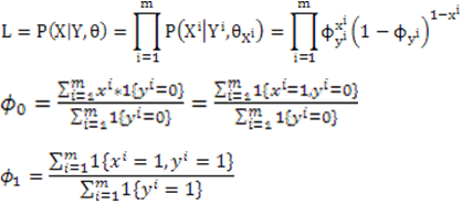
taking the states as in the data. According to the following equations, the log likelihood can be decomposed into sub-log-likelihoods, which are the CPTs of individual r.v.s. Thus the problem is simplified into maximizing the likelihood of each r.v. independently. Now suppose we have a root node Y, and its probability when Y=1 is denoted by sigma. The likelihood of its data can be represented as: And its prior probability when Y=1 can be derived by: Similarly, the conditional probability of a node X dependent on Y can be inferred in the following way.
When a particular set of r.v. instantiations cannot be found in the
data, the estimate of CPT encounters the problem of 0/0. An ad hoc way
to solve this is to add 1 to the denominator, which forms 0/1. However, a probably more intelligent way is to apply smoothing in a similar way of Laplacian smoothing.
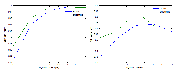
The intuition of the detection method is that if the deviation from the
real answer and the modeled answer is so large that it cannot be
explained by noise, then it is identified as possible deception. The
way I do it is to first calculate the prediction error, which is the
difference between answers from the simulator and answers from the
model. The prediction error serves as an estimate of noise. Assuming
normal distribution, I obtain the standard deviation of prediction
error. If the difference between the deceptive answer and the answer
from the model is beyond four std deviations, then it is identified as
deception. Experiments and Results The network I used as the simulator is an existing BN called Alarm Network. It was originally built to monitor patients with intensive care. It is used in my experiment due to the moderate size. The Alarm Network has 37 nodes, 105 states and 46 arcs. In the experiment, 10, 10^2, 10^3, 10^4 and 10^5 training samples are generated from the simulator respectively. For each size of training sample, a "model" BN is learned and compared with its simulator BN.
After the so called "model" BN is learned, I conduct a probabilistic
inference on it and obtain the posterior probability distribution of
each variable. The learning error is calculated from the
averaged difference between the posterior probability distribution of
the simulator and that of the model over all the variables. I am more
interested in the error in the posterior probability instead of that in
the parameter (CPTs) since in mimicking someone's mind his final
opinion on some event is more important than how he derives the
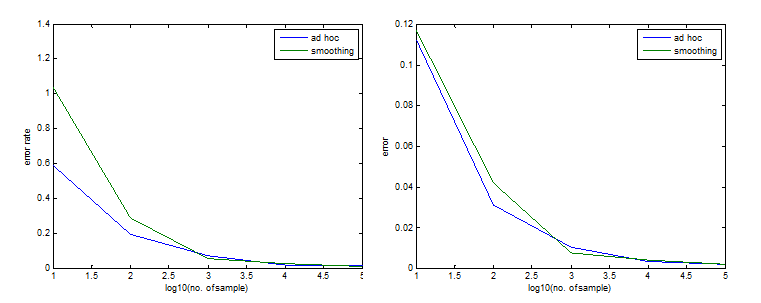
opinion. In the result, I also plot the error rate, which is
(Error)/(posterior probability of the simulator). We can see from
Figure 3 that the error rate is satisfactorily small and decreases as
we have more training data. However, the smoothing method is not as
effective as the ad hoc one at first. It is because the smoothing poses
a strong prior knowledge on the CPTs especially when the data size is
small, and thus the estimation does not depend on the data much and
results in a worse performance. The smoothing starts to take effect
when we have 1,000 data samples, but it is NOT much more effective than
the ad hoc method. It might be because that when the data size is
large, the prior knowledge is not influencing much. Fig. 3 (left) Plot of error rate. (right) Plot of error.
The detection rate increases as the increase of data size. The
detection rate of using smoothing is higher than that of using ad hoc
at first. And since the detection rate is higher, the false alarm rate
is also higher. The influence of smoothing/ad hoc is more significant
when the data size is small, and becomes trivial when the data size is
10,000 and higher. Another observation is that the detection rate does not increase any more after 10,000 samples although the error rate of learning BN still reduces. Timeline The rest of the term will be spent on the study and implementation of the EM algorithm used to learn BN with incomplete observations, and using the implemented detection method and the learned BN to detect deception. |



_text_