
Figure 1: Photo taken and its selected region to be analyzed
The aim of our project is to classify terrain types using information from both a camera and proprioceptive data from the Yeti robot. This use of sensor fusion was decided upon after noting that either sensor suite on its own had its weaknesses, but the fusion of the two would strengthen the classification. For instance, gravel was visually hard to distinguish from pavement and sand, but with proprioceptive data, it became much easier. Similarly, proprioception struggled with distinguishing grass from pavement, but with vision this classification was almost trivial.
After some research and initial trial runs, we have decided to use a Support Vector Machine (SVM) to make our terrain classification (Gurban and Thiran). This decision was based on the fact that SVM's are a supervised learning method that allows for some misclassifications in the data. We realized that a supervised learning method was needed for several reasons. First, since the training data has more than two classes, hand-labeling was needed. More importantly, since the different classes overlap in some cases, supervised learning was imperative. We decided to train a single SVM in our sensor fusion, and simply concatenate data from each sensor for each training data point. We could have trained a SVM for each sensor suite, and then combined them, but we decided that the simpler method of a single SVM would serve our purpose suitably.
Our method begins by taking in vision data in the form of a .jpg file. Our Matlab program loads in the file and takes a section of the photo corresponding to the terrain directly in front the robot to serve as our input to the program. The mean RGB values from the small section of the photo are computed by simply taking the mean of each of R, G, and B. Next, we discovered that converting to YUV (http://en.wikipedia.org/wiki/YUV) color space and ignoring the Y (luminance) component made it much less sensitive to brightness differences and shadows found in our training data set. So we take the mean RGB values of the photo and transform them to YUV values. These mean YUV values are then stored for each photo to be used later in conjunction with the proprioceptive data for terrain classification.
Figure 1: Photo taken and its selected region to be analyzed
The proprioceptive data was collected using the Yeti robot. The robot was driven over the same terrain that our vision data was collected from. The Yeti was commanded to drive at varying speeds over the terrain in order to extract force v slip data from its sensors. The sensors used to approximate slip include an optical velocity sensor and wheel encoders on all four wheels. The relative difference between the encoder data and the optical velocity data give rise to the slip estimate. The force estimate used was found by taking the difference of the optical velocity data to get acceleration, which is proportional to force. We plotted the force v slip estimates for each terrain, and fit a linear model with a zero intercept to each using just the linear region where the majority of points reside. The slope of the fitted line for each terrain was stored to be compared along with the vision data. We expected that the slope would vary from terrain to terrain since some terrains (e.g. sand) would exhibit much higher slips at a given force. While in practice this was generally true, there were also some outliers.
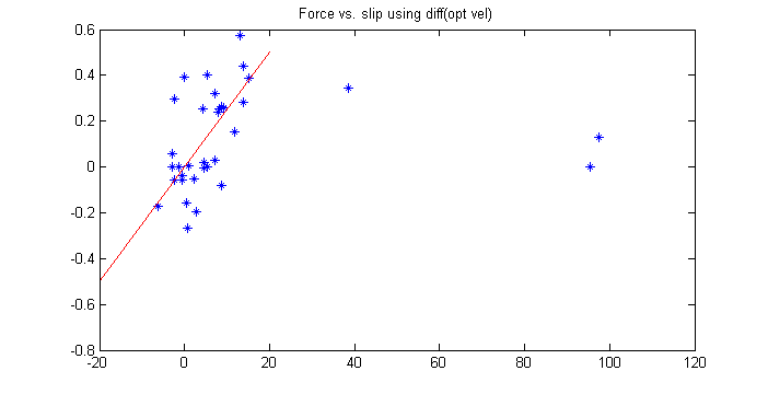
Figure 2: Slope of Force v slip Data for Sand
For our SVM, we mostly used the V data from our vision along with the slope from our proprioceptive data, though we experimented with other options. We found that the data separated nicely along the V axis, but for some terrains and some specific data points had trouble separating along the proprioceptive axis. Where needed we used U and V only for separation.

Figure 3: Data points for all terrains plotted as V color vs slope
The proprioceptive separation issues are most clearly seen for the sand points in yellow. While two of the points have high slopes as expected, there is one data point with a very low slope. The grass data points in green also have some separation along the force vs. slip slope axis. When a SVM was trained to identify the grass points, the classifier did a great job. The SVM also had no problem identifying pavement in black either. The sand and the gravel were a bit trickier since the V color was very close to pavement for the gravel (in magenta) and the sand data points were all over the map for the slope axis.
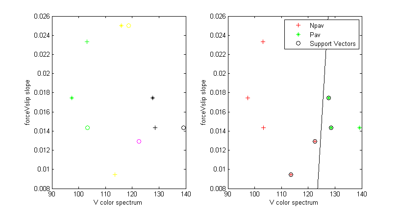
Figure 4: SVM results for Pavement
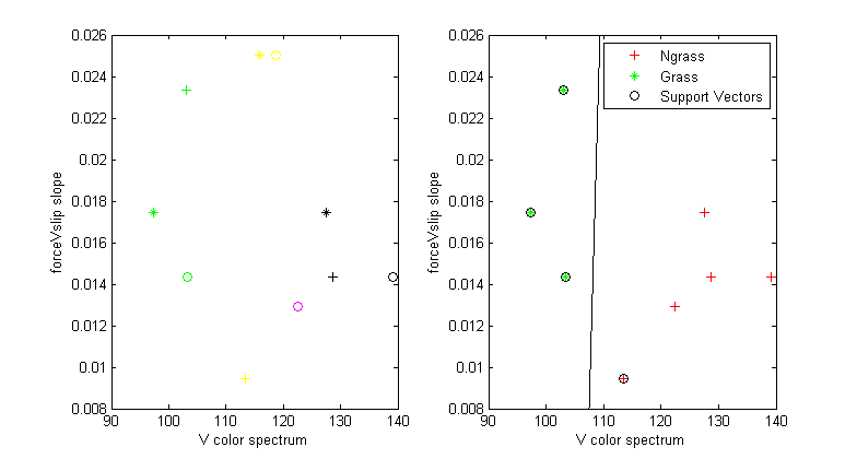
Figure 5: SVM results for Grass
Given these results, we have decided to use a decision tree along with our SVM's in order to make our non-binary classifications. At each node of the tree, we will use our binary SVM to determine whether the given terrain is the terrain in question or not. If not, we test to see if it is another terrain or not using the SVM trained on that terrain. Since we expect that for terrains such as sand and gravel, there will be overlap with other terrains (such as grass and pavement), we hope to use the information higher in the tree to eliminate those points that satisfy the SVM's for those terrains. In the end, we hope to be able to identify all the terrains included in this project.
Currently, the SVM used in our project is the Matlab function svmtain, but we hope to work towards producing our own SVM in Matlab. We have also not yet hand labeled all of our training data, thus accounting for the sparsity in our examples, but this will also be done very soon. Once we have trained all of our SVM's on our training set, we hope to collect data on similar terrains elsewhere on campus to test our method on. These collection sites will include places such as the volleyball court by the Choates for sand, around Thayer and Tuck for grass, and the Thayer parking lot for pavement. We hope to see that the classification process will work just as well on these new unseen terrains.