 |  |  |
| Cook-Torrance | Torrance-Sparrow | Spatially-Varying |
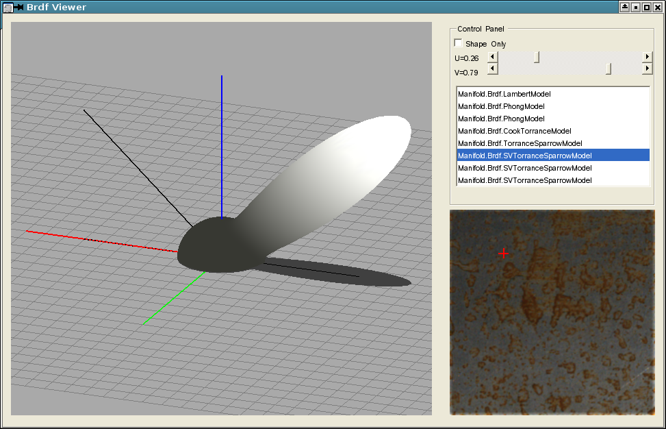
Figure 1: A subset of the implemented BRDF models.
In computer graphics, a Bidirectional Reflection Distribution Function (BRDF) is one of the classic models used describe the appearance property of object surface in computer graphics [PH04]. These functions take in two parameters, ωi and ωo, describing the directions of incoming and outgoing light at the incident point on the material. The result of the function is the fraction of light (called radiance) that is reflected along the specified directions. Because a material acts on light coming in from all directions and out in all directions (cross product of all directions), it is helpful to think of a BRDF as a vector in a high-dimensional space.
In the real world, the physical processes and aging effects that apply to an object vary between different materials, and often have non-linear properties. Thus, linearly blending two BRDFs may generate unnatural results. Physic-based simulations can generate plausible results, but are computationally intensive and require knowledge of underlying physical and biological principles [WTL+06].
Nonlinear dimensionality reduction techniques provide tools to discover underlying structure of the given data without explicitly knowing the function itself, making it possible to approximate a nonlinear appearance manifold from measured spatially- and temporally-varying BRDF data.
Wang et al. [WTL+06] made the observation that the BRDF data is largely self-similar across a material. They conjectured that the BRDF data of a particular material will form clusters in the high-dimensional space of all possible BRDFs, where all the BRDF vectors lie on an appearance manifold. They implemented a variant of Isomap [BST+02] to discover an appearence manifold for a material’s BRDF data.
Our original goals for this project are summarized as the following:
Because we needed a code infrastructure in place to work with the data sets and validate results, we have not met all of the milestone goals from our proposal. However, we believe that we will be able to meet our project goals by the final presentation deadline.
Currently, we are using the Columbia STAF data set of time-varying surface appearance available at http://www1.cs.columbia.edu/CAVE/databases/staf/staf.php. Despite the noise, clamping, and low resolution of the data, there are many benefits to using this data set: large number (26) of types of samples available, the fitted model is easy to work with, and the documentation is adequate. The edges of the data are unusable, so we cropped the data by a 10% margin (using the center 80% of the original width and height, or 64% of the data). The data is time-varying, so we have access to changing, but correlated, information to work with.
We have begun tapping into a local data set of SVBRDFs; this set of data should be of a higher quality, although there are fewer types of samples. We have not yet obtained the data set used by Wang et al. in [WTL+06]. We hope that we’ll be able to use these higher quality data sets for our final presentation.
The BRDF data that we are using and plan to use have been fitted using different BRDF models. The models that we have implemented thus far are Cook-Torrance [CT81], Torrance-Sparrow [TS67], and Oren-Nayar [ON95]. Additionally, we needed a generalized data structure to allow these models to vary over the surface of the material (spatially-varying).
One model that we plan to implement is Ward [War92].
To check the validity of our model implementation, we created a BRDF viewer to view the radiance function given an incident point on the material and an incoming direction. See Figure 1.
| | | |
| Cook-Torrance | Torrance-Sparrow | Spatially-Varying |
We are using the Isomap Matlab code provided by the authors at http://waldron.stanford.edu/~isomap/. We passed to the Isomap algorithm a matrix of distances between every pair of points (our distance metric is described below), along with the option to use k-NN (k = 8) to generate the graph and to reduce to three dimensions. The algorithm returns a set of coordinates for each of the points in the new lower-dimensional space and a set of the constructed edges (between k-NN).
We will be implementing the modified Isomap algorithm and LLE in the next week and will be comparing the resulting manifolds.
While a na�ve approach to these algorithms is to compute a complete distance matrix, we are working on alternative methods to reduce memory usage and computation time.
Our hypothesis is that a good dimensionality reduction will result in a smooth and meaningful manifold for the sampled data. A noisy manifold suggests that either we are reducing the data into too few dimensions, or that our distance metric is not capturing a meaningful distance.
We are currently using the distance metric defined by Pellacini et al. [PL07],

where θi is the angle between the incoming direction and the normal of the surface at the incident point (cos(θi) = |ωi ⋅ N|).
The distance metric used by Wang et al. (defined in [MPBM03]) is slightly different, using log functions. We plan to implement this and compare results.
To estimate the distance between two BRDFs, we use Monte Carlo integration with a large set of pairs of directions (incoming, outgoing) chosen over the normal-aligned hemisphere.
The points and the direction pairs were chosen by Hammersley sequence, a low-discrepancy random sampling algorithm. This low-discrepancy sampling technique allows us to take fewer samples, but still obtain good estimation results. Pseudorandom sampling can form clusters if too few samples are taken.
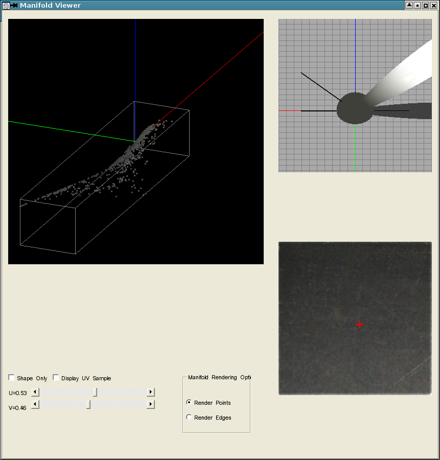
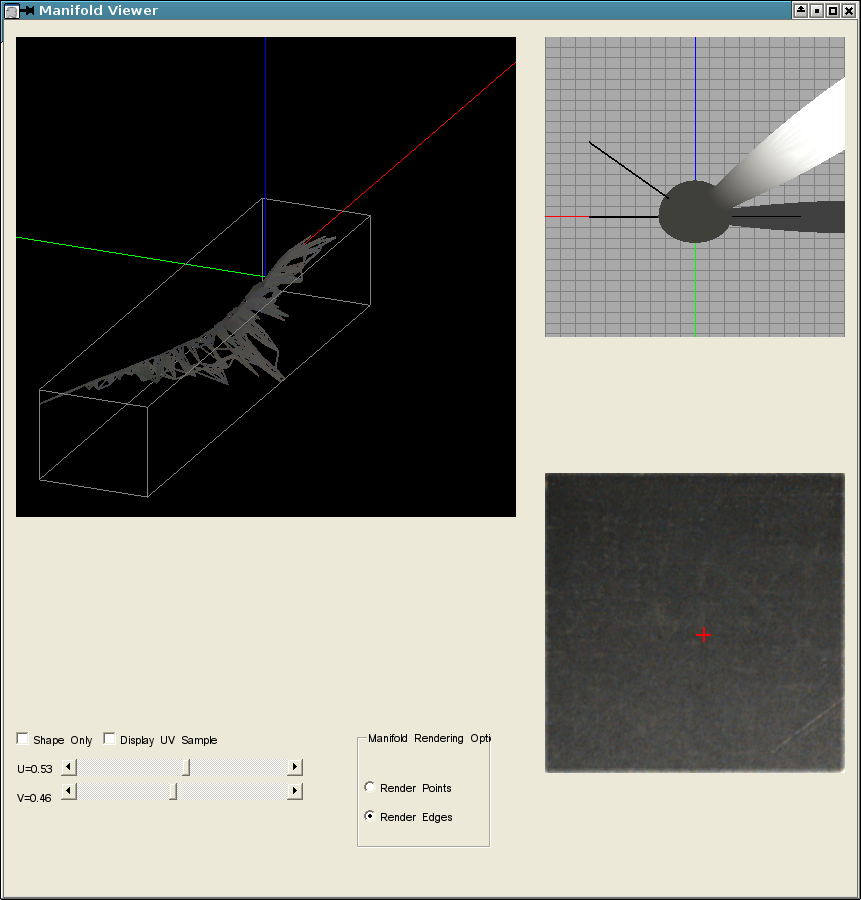
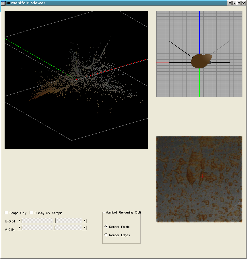
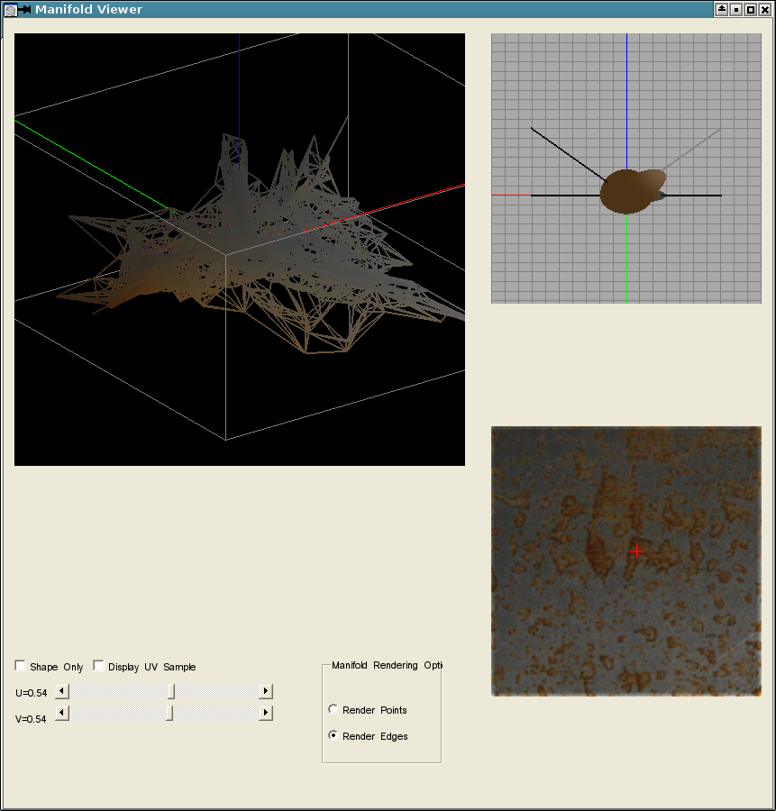
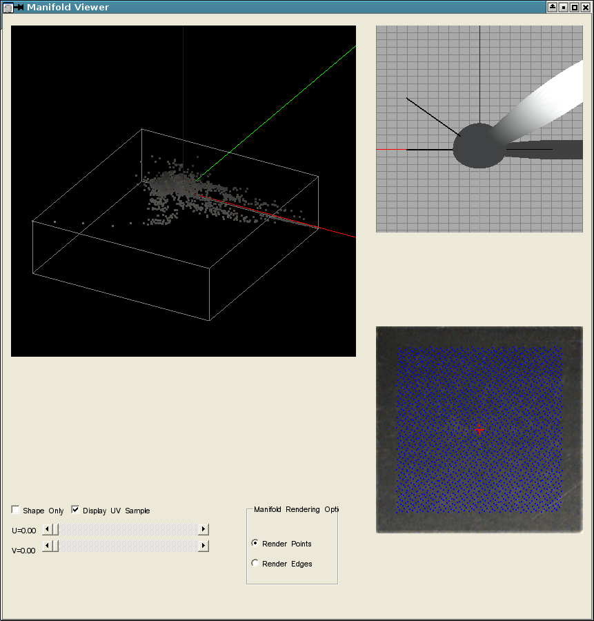
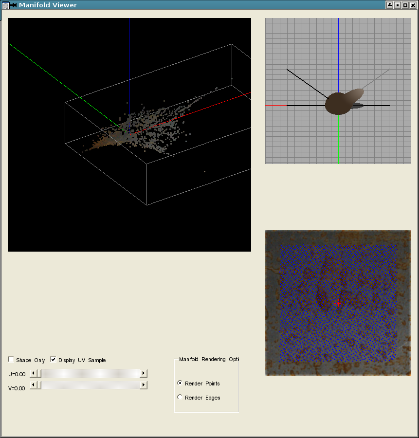
As a sanity check, we implemented a simple manifold viewer. The viewer renders the manifold either by the sampled points or edges between the k-NN. Each point (or the end of the line) is colored according to the corresponding diffuse component of the sample. This render gives a good representation of the appearance manifold.
Matlab does provides a way to view the manifold as a 3D plot but it is not very interactive with the amount of data we’re working on.
The total time for each data set to go through the pipeline is approximately one hour. The pipeline consists of shell scripts, Matlab scripts, and C# code.
With 500 direction pairs, the residual variance for different k values did not change significantly, nor did the appearance of the manifold.
Note: It seems that the manifold is smoother in Figure 3 than in Figure 2. This is either due to the change in sampling or the increase in the number of direction pairs. We will explore this.
 |  |
 |  |
| Points only | Edges |
 |  |
 |  |
| Points only | Edges |
We are planning to implement the modified Isomap algorithm as described by [WTL+06] (k-NN with an ϵ-rule) and the LLE algorithm.
If time allows, we would like to further extend our project to include the following:
| Period | Task |
| Apr. 13 | Proposal & Presentation due |
| Apr. 14 – May 11 | BRDF models. Viz tools. Isomap on 2k samples. |
| May 11 | Milestone Presentation |
| May 12 – May 23 | Implementing LLE, alternative BRDF metric |
| May 20 – May 23 | Work with other data set |
| May 25 – May 30 | Buffer time, polishing result |
| May 25 – May 30 | Buffer time, final report write up |
| Jun. 1 | Final Report |
[BST+02] M. Balasubramanian, E.L. Schwartz, J.B. Tenenbaum, V. de Silva, and J.C. Langford. The isomap algorithm and topological stability. Science, 295(5552):7, 2002.
[CT81] R.L. Cook and K.E. Torrance. A reflectance model for computer graphics. pages 307–316, 1981.
[GVM07] Mike Gashler, Dan Ventura, and Tony Martinez. Iterative non-linear dimensionality reduction by manifold sculpting. Advances in Neural Information Processing Systems, 19, 2007.
[MPBM03] W. Matusik, H. Pfister, M. Brand, and L. McMillan. A data-driven reflectance model. ACM Transactions on Graphics, 22(3):759–769, 2003.
[ON95] M. Oren and S.K. Nayar. Generalization of the Lambertian model and implications for machine vision. International Journal of Computer Vision, 14(3):227–251, 1995.
[PH04] Matt Pharr and Greg Humphreys. Physically Based Rendering: From Theory to Implementation. Morgan Kaufmann Publishers Inc., San Francisco, CA, USA, 2004.
[PL07] F. Pellacini and J. Lawrence. AppWand: editing measured materials using appearance-driven optimization. ACM Transactions on Graphics, 26(3):54, 2007.
[RS00] Sam T. Roweis and Lawrence K. Saul. Nonlinear dimensionality reduction by locally linear embedding. Science, 290(5500):2323–2326, 2000.
[TS67] K.E. Torrance and E.M. Sparrow. Theory for off-specular reflection from roughened surfaces. Journal of the Optical society of America, 57(9):1105–1114, 1967.
[War92] G.J. Ward. Measuring and modeling anisotropic reflection. ACM SIGGRAPH Computer Graphics, 26(2):272, 1992.
[WTL+06] Jiaping Wang, Xin Tong, Stephen Lin, Minghao Pan, Chao Wang, Hujun Bao, Baining Guo, and Heung-Yeung Shum. Appearance manifolds for modeling time-variant appearance of materials. ACM Transactions on Graphics, 25(3):754–761, July 2006.