Classifier Performance
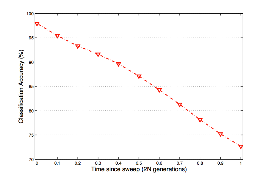
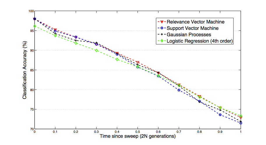
Fig. 1: The best results for each classifier show that fairly similar accuracy can be achieved. Logistic regression with a 4th order basis function performed most poorly at time 0, however it was the best performer at t=1.0.
Logistic Regression
Classification via logistic regression was attempted using 4 basis functions: Linear, 2nd, 3rd and 4th order polynomials (Fig. 2). The 4th order polynomial was the best model tested within this algorithm, however, at time = 0 logistic regression was the poorest performer of all the classifiers examined (Fig. 1). Interestingly, 4th order logistic regression was the best performing method at time =1.0 (Fig. 1). ROC plots show that false positive rate decreases as the order of polynomial increases, as do the AUCs (Fig. 3). Interestingly, again, was that AUC values for 2nd, 3rd, and 4th order basis functions were higher across all time than was SVM, RVM and GP methods, even though logistic regression classification accuracy was poorer (FIg. 3,
Data
Using coalescent simulation software, I have generated data sets containing 1,089,000 events for each class of sweep. Each class is further defined by the time since the sweep occurred, thus each class is represented by 99,000 events at time points 0.0 - 1.0, at an interval of 0.1. A unit of time is defined as 2*N generations, where N represents the population size; time 0.0 describes the generation immediately following a sweep. We assume a fixed population size throughout the experiment.
For each classification algorithm, training took place on 20,000 examples (10,000 of each class) at each time point. Testing was done on 178,000 examples (89,000 of each class) at each time point.

Fig. 2: Training results for logistic regression. Accuracy improved as the order of polynomial basis function increased, peaking at 4th order and decreasing at 5th, 6th and 7th order.
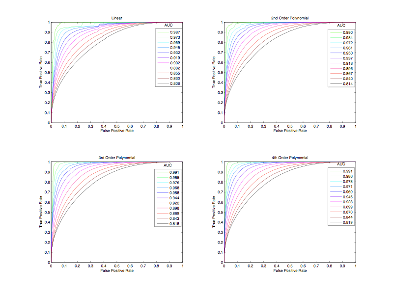
Fig. 3: ROC and AUC data for logistic regression testing data. Colors represent time steps, from light green (time 0) to black (time 1).
Gaussian Processes
While testing gaussian processes on 2500 examples and testing on a full dataset proved that classification was not only possible, but also as accurate as other methods, convergence was not obtainable on the full training dataset. The most accurate classification was achieved using the following parameters: Mean function - “meanConst” (constant mean function, Covariance function - “SEard” (squared exponential covariance function with “Automatic Relevance Determination”), Likelihood function - “likErf” (error function for binary classification), Inference method - “infLaplace” (Laplace approximation to the posterior gaussian process). Training and testing using gaussian processes was also the slowest of the 4 classifiers.
All gaussian process experimentation was performed using GPML v3.1 in Matlab 7.11.0 (R2010b).
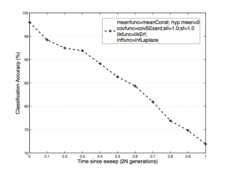
Fig. 4: The slowest of the 4 methods, Gaussian Processes proved to be an accurate tool for classification. The classifier was learned on 1500 examples, unlike the rest of the classifiers, as convergence on full training sets was not possible to obtain.
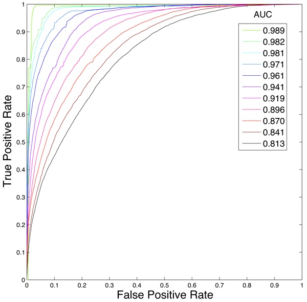
Fig. 5: Gaussian Processes’ ROC and AUC scores.
Support Vector Machine
Using LIBSVM v3.1 with the matlab front end, I trained and tested on the full datasets. Classification was very good through time point 0.5, then tailed off, relative to other methods. Best accuracy was obtained using the Radial Basis Function Kernel, C=1, and h = 0 (turn off shrinking heuristics). The SVM classifier was the 2nd fastest method tested, training on 242,000 examples and testing on 1,936,000 examples in 2121.66 seconds (~35 minutes).

Fig. 6: SVM performance was excellent until time point 0.5 (see Fig. 1). SVMs were the 2nd fastest of the tested algorithms.
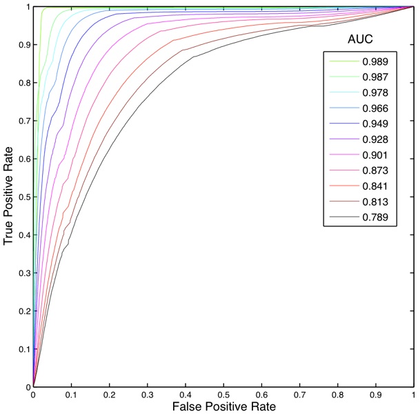
Fig. 7: ROC and AUC for SVM using RBF kernel and C=1.
Relevance Vector Machine
The last classifier I experimented with was the Relevance Vector Machine, which is actually a type of Gaussian Process. This method not only produced the most accurate testing rate, it was also the fastest of the methods I examined (train and test on all data points for each time step in ~ 8 seconds). All RVM training and testing was done using the “Sparse Bayes” engine.
Fig. 8: The Relevance Vector Machine was the fastest and most accurate (except t=1 *see Fig. 1 and Logistic Regression*) of all methods I utilized.
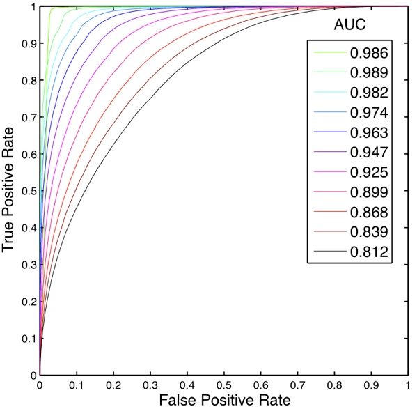
Fig. 9: RVM ROC and AUC plots showed excellent performance, comparable to most of the other methods examined.
Remarks / Conclusion
Through this experiment, I have shown that it is possible to accurately classify nucleotide fixations using a wide variety of machine learning methods, over a range of time points. While I have been able to achieve a high classification accuracy at early time points, this accuracy does decrease as a function of time. This is to be expected, as the signal which enables classification in the first place deteriorates through the process of recombination.
Considering the merits of each classifier, the next phase of this project will center on the use of SVMs and RVMs. Phase II will bring new data statistics into the fold, as well as attempting to use the classifiers learned on simulated data to classify real world population data.
Another interesting possibility, addressed during the Milestone report, is the potential to conduct training on raw, unconverted simulation data. This method, as noted, has the potential to radically increase the feature space, and perhaps improve classification accuracy.
Special thanks to Professors Andy Kern and Lorenzo Torresani for their help, advice and encouragement.