Smart Stock Selection
Final Report

Chanjuan Wen

May 31, 2011

1 Introduction

Stock represents a portion of ownership of a company. Distinct from the property and the assets of a business, stock could fluctuate in quantity and value[1]. For stock traders, fluctuation in stock’s price directly determine their profit or loss. Therefore, to maximize the profit, it is of great value to choose those stocks with high return. Stock market prediction is to determine the future price of a company stock or other financial products traded on a financial exchange[2]. Obviously, successful stock prediction can yield significant profit. However, accurately predicting the performance of a stock is very difficult for the following reasons:

Public stock data is limited. The key to accurate analysis of stocks’ performance is the availability of high quality financial data. For individual stock traders, high quality financial data is usually too expensive to get. For example, we can only get the daily open price, close price, and trading volume of a stock.
Influencing factors are too many to consider. The performance of a stock can be influenced by a lot of factors, such as the company’s coming event, revenue, stock traders’ activities, etc. Besides, each stock has many properties, including the company’s total asset, annual revenue, etc. The underlying relations between those factors, properties, and performane is very hard to figure out.

But many past studies has showed that stock returns are predictable based on historical information of that stock[3]. Many researchers apply machine learning techniques to stock prediction. Avramov and Chordia’s work showed that returns on individual stocks are predictable[4]. Hamid and Iqbal[5] used neural networks for forecasting volatility of the S&P 500 Index futures options. Comparing to statistical methods, Machine Learning Methods don’t involve assumptions about the distribution of dataset, thus are very suitable for stock prediction[3].

Since long term invesetment(months or years) requres fundamental analysis of the company’s performance and financial record, and super short-term (1-2 days) investment will be only available to large financial coorperation due to the high commission fee and need high quality financial data, in this project, I mainly focus on short-term stock trading (1-2 weeks).

So, the goal of this project is to help investors make short-term stock investment by constructing a profitable stock portfolio using machine learning techniques. A portfolio is a set of stocks the investor will hold in a prerid of time. An investor is able to gain money by buying stocks in low price and selling them in higher price. To maximize the profit of a profolio, investors need to select stocks with a high return rate. Let V_i denote the initial value of an investment, and V_f denote the final value of it, then the return rate is[6]:

r_arith = (V_f − V_i)/(V_i)

2 Previous Work

Previous work on stock prediction mainly falls into several categories as follows:

Predict the price trend of individual stocks. In this category, classification algorithms such as SVM are used to predict whether the price of some stock will go up or down in certain future time. However, this type of prediction is not that useful because it does not reflect the amount of change. For example, a stock with 0.01% increase in price and one with 100% increase in price will both be predicted as going up. Obviously, a stock with 0.01% increase is not as profitable as the one with 100% increase.
Predict the exact price of individual stocks. Pham et al[7] used deep correlation algorithm to predict the next day’s price of individual stocks based on today’s information of stock trading. This type of prediction mainly focus on minimizing the overall average prediction error, which is not suitable for my task, since the goal here is to identify high return rate stocks. The prediction errors of low return stocks and negtive return stocks are not important.
Predict the exact stock index. Related work, such Theodore and Huseyin[8], includes using SVM for the whole stock forecasting, i.e., pridicting the exact stock index. For individual stock traders, the exact stock index is not useful for stock selection because the increase of the whole stock market’s index does not neccessarily mean the increase of individual stocks. Moreover, the stocks we want to choose have to outperform the stock index. Otherwise, we can just buy the stock index.

3 Objective

As analyzed previously, the return of a stock directly reflects the amount of profit, and thus has a significant economic value. By assuming no commission cost for trading stocks, my objective of this project is to select stocks to form a portfolio with high return. For each week t, based on the historic trading information prior to week t, the return rate for each stock is predicted and each stock is assigned a rank based on its predicted return. Then we chose N stocks with the highest rank to form the portfolio of size N for week t.

4 Approach

4.1 Competitive Learning Based Non-parametric Model

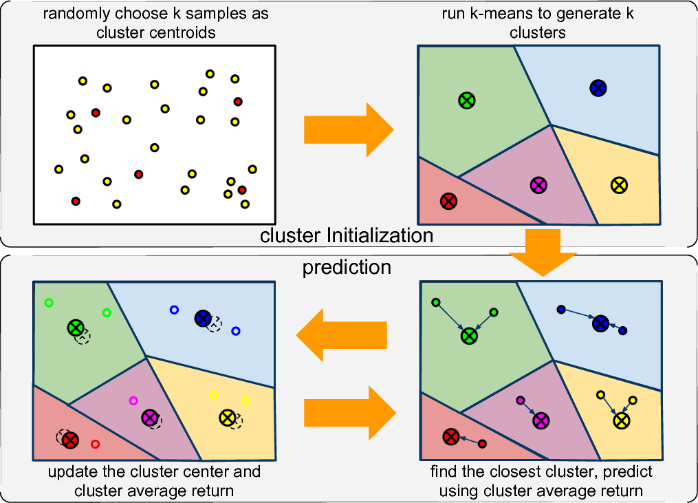
Since we have a very large dataset and the data grows every trading day, I want my model to grow with the data. So, I used a non-parametric model based on a competitive learning method[9]. As illustrated in the below figure, my algorithm is composed of three steps as follows:

Cluster Initialization. Firstly, in the 3-D feature sample space, I randomly choose k samples as the cluster centers. Then in the K-means method, firstly, for each feature sample, I calculate its distance to every cluster center and choose the closest cluster to label it. Then by fixing the cluster label of each feature sample, I update the cluster center by averaging all the feature vector belonging to that cluster. By repeat this process until convergence, I can get k cluster. Meanwhile, for each cluster center, the average feature vector and weekly return are also recorded. After getting the k clusters, I use the feature vectors of the k cluster centers to construct a Kd-Tree for nearest neighbor search in the prediction stage.
Return Prediction. For each stock i in week t denoted by x⁽ⁱ⁾_t, I use Kd-Tree to find its nearest cluster c, and use c’s average return as the predicted return for x⁽ⁱ⁾_t. After predicting the weekly return for all stocks, I choose N stocks with the highest return to form the portfolio.
Cluster Update. At the end of week t, we have the actual return of all stocks for week t. So, we can update the clusters. There are two things needed to update as follows:
- Update the cluster centers. For each stock i, I use its feature vector to update the center of cluster which i belongs to. Let x^j_avg denote the average feature vector of cluster j, n denote the number of feature samples belonging to j, then the update equation is: x^j_avg = (x^j_avg*n + x⁽ⁱ⁾_t)/(n + 1).
- Update the average return of each cluster. For each stock i, I use i’s actual return at week t to update the average return of cluster which i belongs to. Let r^j_avg denote the average return of cluster j, n denote the number of feature samples belonging to j, then the update equation is: r^j_avg = (r^j_avg*n + r⁽ⁱ⁾_t)/(n + 1).

Figure 1 Three steps of my algorithm

4.2 Other Models for Comparison

To measure the economic profit by using my method for weekly return prediction, I also implement another two models to be the control group: Linear Regression and Nonlinear Regression. They are decribed in details in the following two subsections.

4.2.1 Linear Regression

As one of the supervised learning algorithm, linear Regression uses a linear functions to model the relationship between a scalar variable y and multiple variables X[10]. The linear function is usually in the following form:

f_θ(x) = θ₀ + θ₁x₁ + θ₂x₂ + ⋯ + θ_nx_n

Here, the θ_i’s are the parameters parameterizing the space of linear functions mapping from X to Y[11]. Given a training set, we choose θ_i’s which can minimize the sum of squared differences error denoted as follows:

E(θ) = (1)/(2)^m⎲⎳_i = 1(f_θ(x⁽ⁱ⁾) − y⁽ⁱ⁾)²

4.2.2 Nonlinear Regression

To avoid underfitting may caused by Linear Regression, Nonlinear Regression uses a nonlinear combination of the model parameters and depends on multiple independent variables X[12]. The nonlinear function I choose is in the following form:

f_θ(x) = θ₀ + θ₁x₁ + ⋯ + θ_nx_n + θ_n + 1x²₁ + ⋯ + θ_2nx₁x_n + θ_2n + 1x²₂ + ⋯θ_3n − 1x₂x_n + ⋯ + θ_{((n + 1)(n + 2))/(2)}x²_n

Similar to Linear Regression, we choose θ_i’s which minimize the sum of squared differences errors. Since some nonlinear functions may cause overfitting while some other may cause underfitting, choosing a good nonlinear function is very important.

5 Experiment

5.1 Data Retrieving

Using Yahoo Stock API, I collected the historic data of all stocks in S&P 500 index from April 2001 to April 2011. For each trading day in that period, I retrieve the daily price and trading volume of each stock. After omitting stocks with missing data, the final dataset includes the daily price and trading volume of 462 stocks for 2515 days.

5.2 Data Preprocessing

In this project, I choose to predict the weekly return, instead of daily return, of each stock. So, I pad the trading days into weeks. Each week is composed of five trading days. Let R(t) denote the return of week t, d denote the last day before week t, p(d) denote the price of day d, and V(t) denote the total trading volume of week t. Then we have:

R(t) = (p(d + 5) − p(d))/(p(d)) V(t) = ^d + 5⎲⎳_{j = d + 1}v(j)

So, after preprocessing, my dataset includes 500 weeks data of 462 stocks.

5.3 Feature Selection

As discussed in the previous section, the prediction for return of week t is based on the actual return and trading volume of week t − 1 and t − 2. So, for the following three methods, I choose difference feature vectors.

Competitive learning based non-parametric Model. As stated in Cooper’s work[13], to predict the return of week t, I choose the actual return of week t − 2 and t − 1, and the volume value ratio, denoted by VR(t) to compose the feature vector. The volume value ratio and feature vector for my method is:

x⁽ⁱ⁾_t = [R⁽ⁱ⁾(t − 2), R⁽ⁱ⁾(t − 1), (V⁽ⁱ⁾(t − 1) − V⁽ⁱ⁾(t − 2))/(V⁽ⁱ⁾(t − 2))]
Linear Regression. In this method, I simply merge the actual return and trading volume of the previous two weeks. Since the trading volume is usually more the order of 10⁶ which is much more than the price, to avoid numerical precision issues in computation, I transform the trading volume values using a scaling factor which we set to be 10⁶. Let α denote the scaline factor, then the feature vector for the Linear Regression model is

x⁽ⁱ⁾_t = [1, R⁽ⁱ⁾(t − 2), V⁽ⁱ⁾(t − 2) ⁄ α, R⁽ⁱ⁾(t − 1), V⁽ⁱ⁾(t − 1) ⁄ α]
Nonlinear Regression. Similar to the Linear Regression, for this method, I choose the actual return and trading volume of the previous two weeks. The difference is that I use a quadratic function to generate the feature vector for the Nonlinear Regression model.

x⁽ⁱ⁾_t = [1, x₁, ⋯, x₄, x²₁, x₁x₂, ⋯, x₁x₄, x²₂, x₂x₃, ⋯, x₂x₄, ⋯, x²₄] x₁ = R⁽ⁱ⁾(t − 2) x₂ = V⁽ⁱ⁾(t − 2) ⁄ α x₃ = R⁽ⁱ⁾(t − 1) x₄ = V⁽ⁱ⁾(t − 1) ⁄ α

5.4 Parameter Configuration

In 500 weeks historic data of 462 stocks, I choose the first 149 weeks data as the training set, and the rest 351 weeks data as the test set. About the portfolio size, the experiments showed that N = 10 is a good portfio size which can yield pretty high return. Similarly, I also did several test for the number of clusters and found that k = 50 is a good choice.

6 Results

To show the performance of my algorithm, I plot the cumulative return with respect to the increasing number of weeks. As illustrated in the below figure, the x-axis represents the number of weeks, and the y-axis represents the cumulative weekly return rate. The red curve denotes the performance my algorithm, and the yellow and green curves denote that of the linear model and nonlinear model separately. As we can see, my algorithm performs much better than the linear regression model and nonlinear regression model.

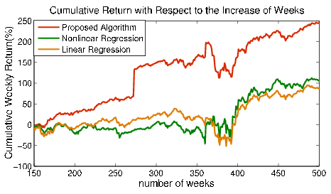
Figure 2 Cumulative Return with Respect to the Increase of Weeks

7 Conclusion

From the dataset tested, we can conclude that the portfolio constructed by my non-parametric model consistently yield higher cumulative return than those constructed by the linear regression and non-linear regression model. In a time period of 7 years, using my model to select stocks for each week can achieve 250% cumulative return.

References

[1] http://en.wikipedia.org/wiki/Stock

[2] http://en.wikipedia.org/wiki/Stock_market_prediction

[3] Robert J. Y, John N., Charles X. L. Application of Machine Learning to Short-term Equity Return Prediction. 2006.

[4] Avramov D., Chordia T. Predicting stock returns, Journal of Financial Economics 82, 387-415. 2006.

[5] Hamid S.A., Iqbal Z. Using neural networks for forecasting volatility of S&P 500 Index futures prices, Journal of Business Research 57, 1116-1125. 2004.

[6] http://en.wikipedia.org/wiki/Rate_of_return

[7] Hung P., Andrew C., Youngwhan L. A Framework for Stock Prediction. 2009

[8] Theodore B. T., Huseyin I. Support vector machine for regression and applications to ﬁnancial forecasting. IJCNN2000, 348-353.

[9] Robert J.Y, Charies X.L. Machine Learning for Stock Selection. The 13th ACM SIGKDD international conference on knowledge discovery and data mining. New York, USA, 2007: 1038-1042

[10] http://en.wikipedia.org/wiki/Linear_regression

[11] http://www.stanford.edu/class/cs229/notes

[12] http://en.wikipedia.org/wiki/Nonlinear_regression

[13] Cooper M. Filter ruies based on price and volume in individual security overreaction. Review of Financial Studies, 1999(2): 901-935

Smart Stock Selection Final Report