Reinforcement Learning in Coevolution Models

QINXIN PAN

Abstract

Most biological networks such as gene regulatory networks, protein interaction networks show scale free structure. The scale free property make the networks more robust to environmental perturbations. Moreover, there might be a potential evolutionary advantage. In this study, I try to address whether scale free networks have any advantage in the context of coevolution. From the preliminary results, the scale free networks tend to evolve better and faster than random networks. Moreover, the evolvability is more robust to the change of average connectivity.

1. Introduction

1.1 Coevolution

Coevolution is the change of a biological object triggered by the change of a related object. Two post well known relationships are competition and collaboration. Here I focused on the collaboration relationship, which means two individuals from different I addressed the question that whether the scale free topological structure brings the networks any advantages in coevolution. population will collaborate to finish a larger task.

1.2 Random Boolean Network

A Boolean network consists of a set of Boolean variables whose state is determined by other variables in the network. Since their proposal in 1969, RBN have successfully described in a qualitative way several important aspects of the gene regulation and cell differentiation process. In this study, I use threshold RBN.

1.3 Scale free

Scale free structure is a topological property in whcih very few nodes( hubs) have many edges whereas most nodes have only 1 or 2 edges.

2. Methods

2.1 Constructing networks

I used threshold RBN. Each node represents a gene. It is either 1 or 0, which means the gene is expressed or not. The directed edges indicate the regulating relationships. For each node, its state at next time point will be decided by its regulators’ states at current time point. Given the initial state, the networks will fall into a cycle eventually and display that cycle repeatedly after as shown in figure below.

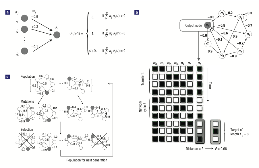
Figure1. The dynamics& Evolution of networks. Network Construction and Evolutionary Algorithm. (a) Each node has its regulators and each weight has a weight uniformly distributed between (-1,1). For each node, the state at next time point will be decided by the weight of its coming in edges and the states of its regulators at current time point. (b) For one network, given the initial configuration, it will reach its attractor at certain point and start repeating. Choose one node as output node randomly, define its states in the attractor as output of network. Set an arbitrary binary sequence as target function, fitness can be measured based on the hamming distance between output of the network and the target function. (c)shows how the mutation work in the evolutionary algorithm. Mutations can happen on both edge existence and edge weights with fixed probability u=0.02. One individual at mother generation will generate 3 mutated offsprings. Together with the mother itself, the 4 networks will go through a tournament and the one with best fitness will be copied to the daughter generation. (Figure from Oikonomou etc.)

2.2 Evolutionary algorithm

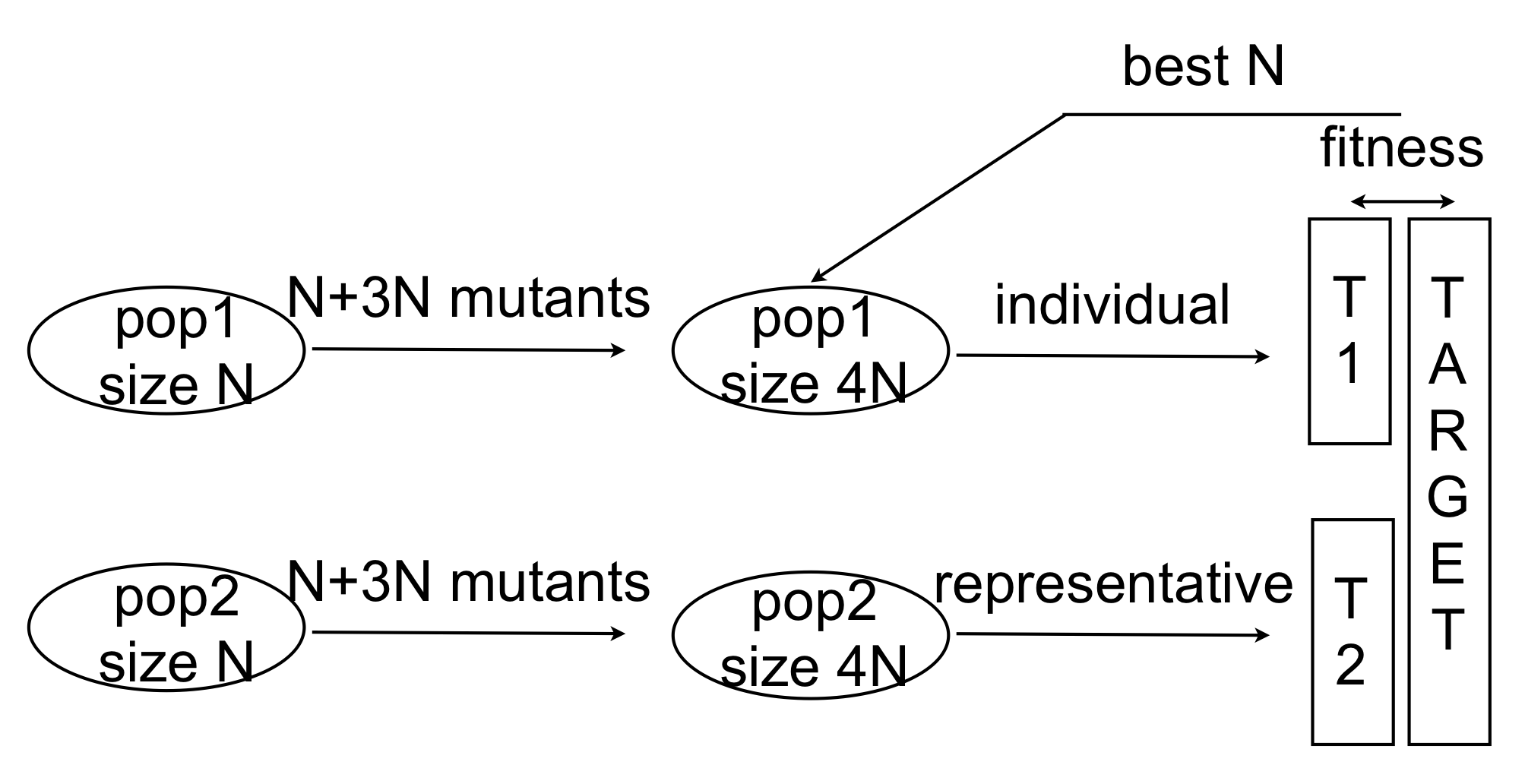
Figure2. The evolutionary algorithm. The two populations start both at size N. After each individual generates 3 mutants, the population size will expand to 4N. The combinations of output from pop1 and output from pop2 mimic the collaborative coevolution relationship. Fitness is calculated according to hamming distance between output and target function. The individuals with higher fitness will be selected into next generation.

2.3 Mutation

Every individual generates 3 mutants with fixed mutation rate 0.02. Each mutation event can either be edge change or edge weight change shown as Figure1c.

3. Results

3.1 Constructing networks with scale free structure.

For the scale free networks, the in degree distribution follows a power law distribution with parameter gamma. For the random networks, the in degree is fixed with parameter K.

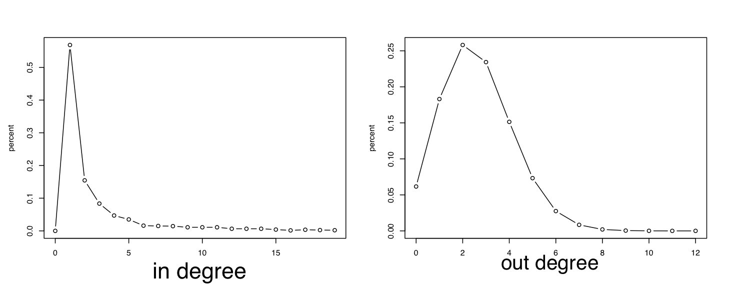
Figure3. The out&in degree distribution of the networks constructed. Each population has 50 networks and each network has 30 nodes.

3.2 Coevolution of networks with different topology structure.

The figure below is a comparision of fitness between scalefree networks and random networks. The preliminary results show that the scalefree networks might be better and faster at evolving.

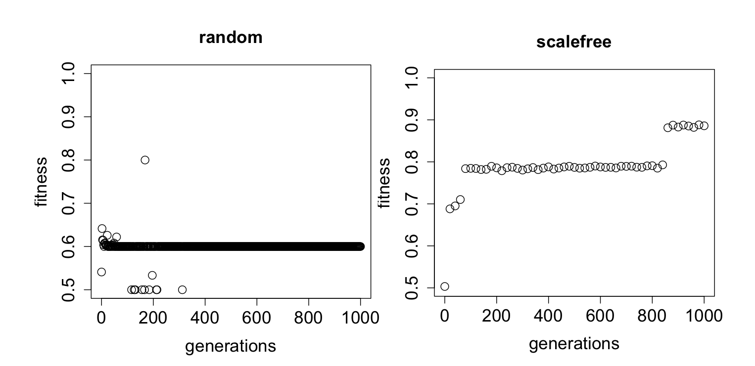
Figure4. The evolution of random & scalefree networks. Data shown are representative run. Each population has 100 networks and each network has 100 nodes.

3.3 How reducing average connectivity influence evolvability?

The figure below show the fitness during evolution with different average connectivity and different structure. From preliminary results, the scale free networks might be more robust to the decrease of average connectivity where as random networks are highly influenced by average connectivity. But this is really preliminary and need more validation.

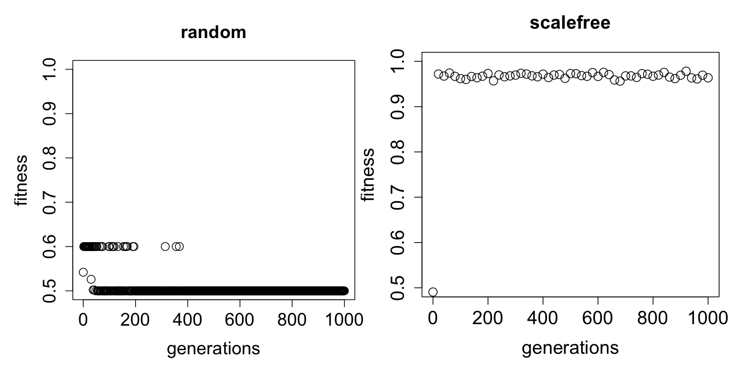
Figure5. The evolution of random & scalefree networks with lower average connectivity. Data shown are representative run. Each population has 100 networks and each network has 100 nodes.

4. Discussion

This study show that there might be an advantage in coevolution for scalefree networks but it needs more experiments to confirm. In the future, I plan to extend this work by using different measurements of evolvability, trying different coevolution relationship etc. Analyzing the possible reason for this advantage will also be interesting.

5.Referrence

Figurea,b, c are from Oikonomou et al.

Oikonomou and Philippe Cluzel,Effects of topology on network evolution. Nature Physics 2, 532 - 536 (2006)

W.Daniel Hillis, Co-evolving parasites improve simulated evolution as an optimized procedure. Physica D: Nonlinear Phenomena 42, 228 - 234 (1990)

Maximino Aldada et al, Robustness and evolvability in genetic regulatory networks. Journal of Theoretical Biology 245, 433 - 448. (2007)