On Using an Autonomous Polar Rover for Machine Learning Based Crevasse Detection

Overview of Motivation and Goals

The purpose of this project is to apply current/new machine learning algorithms to ground penetrating radar data in order to interpret and classify reflection signals. A crevasse is a crack in a glacier posing hazards to NSF Over-snow Traverse vehicles, which are crucial to the mission of supporting science in Polar regions. Though successful,the current methods impose great risk to both man and machine, and are unreliable. We propose an autonomous, GPR towing mobile robot, named Yeti, to carry out crevasse detection surveys. A proposed survey route will be accessed by Yeti as GPS waypoints, and he will explore this route by continuously analyzing the GPR data generated by the unit in his tow. This analysis will be based on image processing and machine learning in order to "decide" whether a radar profile constitutes a crevasse, or safe snow for crossing.

Data

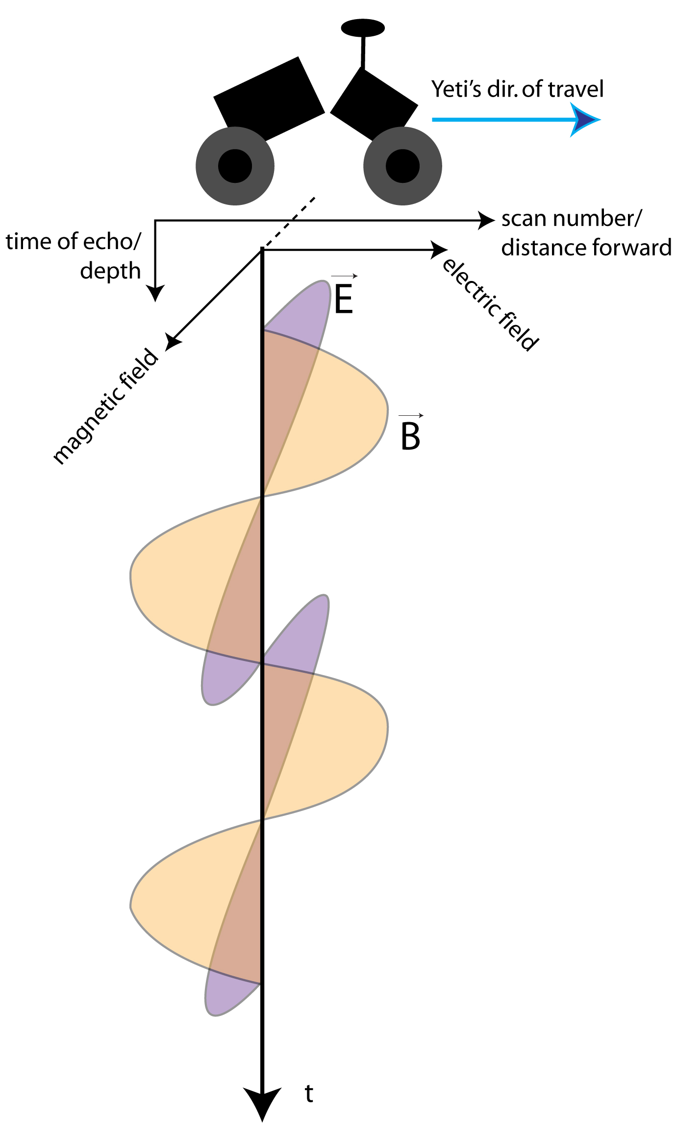
The structure of the data is interesting, in that both axes can be translated into other units, eliminating or creating a time-dependence. For example, for a general radargram, the x axis is "scan number," which is simply a vector of amplitudes received by the receiver during the time window (120 ns). However, since the radar unit is moving at a known, fixed speed (usually 3 mi/h), the units on the x-axis can also be distance. Similarly, the y-axis represents "time," referring to the time each reflection from below is arriving at the receiver. Again, knowing the time window mentioned above, and the dielectric constant of snow/ice, these units can be converted to depth. All of our radargrams have depths of 12.5 m for 30 cm depth resolution. This point is important because it may affect the necessity of algorithms that can handle sequential data.

1. The first is strong, hyperbolic diffractions from the interface between two media with differing dielectric constants. Their hyperbolic shape originates from the type and orientation of radar antennae used. The current model has two dipole bowtie antennae, and their fields are oriented such that energy is preferentially aimed in the forward and backward directions, and its maximum pointed straight down, perpendicular to the ground. The projection of the resulting "cone" of energy resembles an elongated ellipse. This means that, when travelling forward toward a feature in the ground, the energy from the transmitter will reach the feature before the actual radar unit, reflecting back amplitudes proportional to its distance from the GPR. As the radar gets closer to an underground feature, it's reflections increase in both amplitude, and time to echo back, and therefore they also appear closer to the surface.

2. The second corresponds to the void of air enclosed within the crevasse. As the radar eventually reaches the spot directly over the void of the crevasse, a prominent decrease in return signal amplitude occurs, and corresponds to the width of the crevasse. This data pattern is symmetric about the crevasse. This pattern could be characterized by a power value, such as power spectral density, which does not require fourier transforms. This method may be more successful than a simple amplitude threshold approach, as snow density, water content, and other parameters often change throughout a glacier.

3. The third is presence and state of a "snow bridge." After a new crevasse forms, the winter accumulation period allows snow to drift over the opening, and harden. After several iterations of this, a bridge of snow will form accross the opening. As the crevasse ages, this bridge may begin to sag due to increasing weight in the middle, and may eventually break, causing complex inner geometry of the void. Snow bridges are characterized by a continuance of the smooth undulating reflections consistent with debris and crevasse-free snow and firn. In these layers, the dynamic range of amplitudes is greatly reduced, and reflections are slow and wave-like, with zero average slope.

Learning

The goal of learning in this context is to analyze incoming GPR data, and make a decision about whether the data represents a crevasse, or a crevasse-free area. In essence it is a binary classifier, though more classes will be added later in the author's PhD research. These classes would include "crevasse thin enough to cross" vs. "crevasse width too great to cross" and "crevasse at shallow strike angle" vs. "crevasse at near-perpindicular."

To the author's knowledge at this point, there are two main learning algorithms that show promise. A support vector machine based classifier would be useful if performed on a "slice" of GPR data [3]. A slice of data would constitute a certain distance travelled by the radar, and the depth reached by the GPR. The slice would be a matrix of reflection amplitudes at increasing, fixed units of time/distance.

The second interesting algorithm is a Hidden Markov Model (HMM). HMMs are used when data has a sequential nature, and time dependence is required. As mentioned above, this may or may not apply to the GPR data, as the time dimension is not necessarily the most useful to work in. Several studies have been done on HMMs for landmine detection with GPR [1,2]. If we were to consider each vector of reflection amplitudes as one slice of data, with a time component satisfied by the markov model, the algorithm would hopefully consider the order of features, or observables, present in order to classify an area.

Milestone Report

A deeper look at the data

The novelty of this topic is such that databases of any kind have not been created. The data used for this project has only recently become available, straight from the ice cap. The GPR control unit has a 64 Mb internal memorry buffer, which immediately writes the data to a flash card. The data consis of raw electromagnetic energy amplitude values(in Volts) that are incident upon the receiving antenna, within a 120 nanosecond time window. Each time a signal is recorded by the receiver, it's time of arrival is also recorded, and knowing the relative speed of radar waves through ice, the y-axis can be represented as depth. In a given "scan" (vector of amplitudes), the reflected signal can be plotted as amplitude vs. depth, amplitude vs. depth vs. distance. The most useful view for human operators thus far has been a color map, where time is on the x-axis, depth on the y-axis, and amplitude of reflected signal represented in value by a color/gray value. However, time can also be converted to distance, but we can see that distance would not be a useful measure, as there would be no reference point if implemented in real time, as is the eventual goal. The typical size of a data matrix corresponding to "one" crevasse, meaning both the void and the indicating hyperbollic diffractions, is 512x500. The receiving antenna takes 512 amplitude and return time samples every 1/40th of a second. This size matrix is roughly equal to a 12.5x5m area of snow and firn.

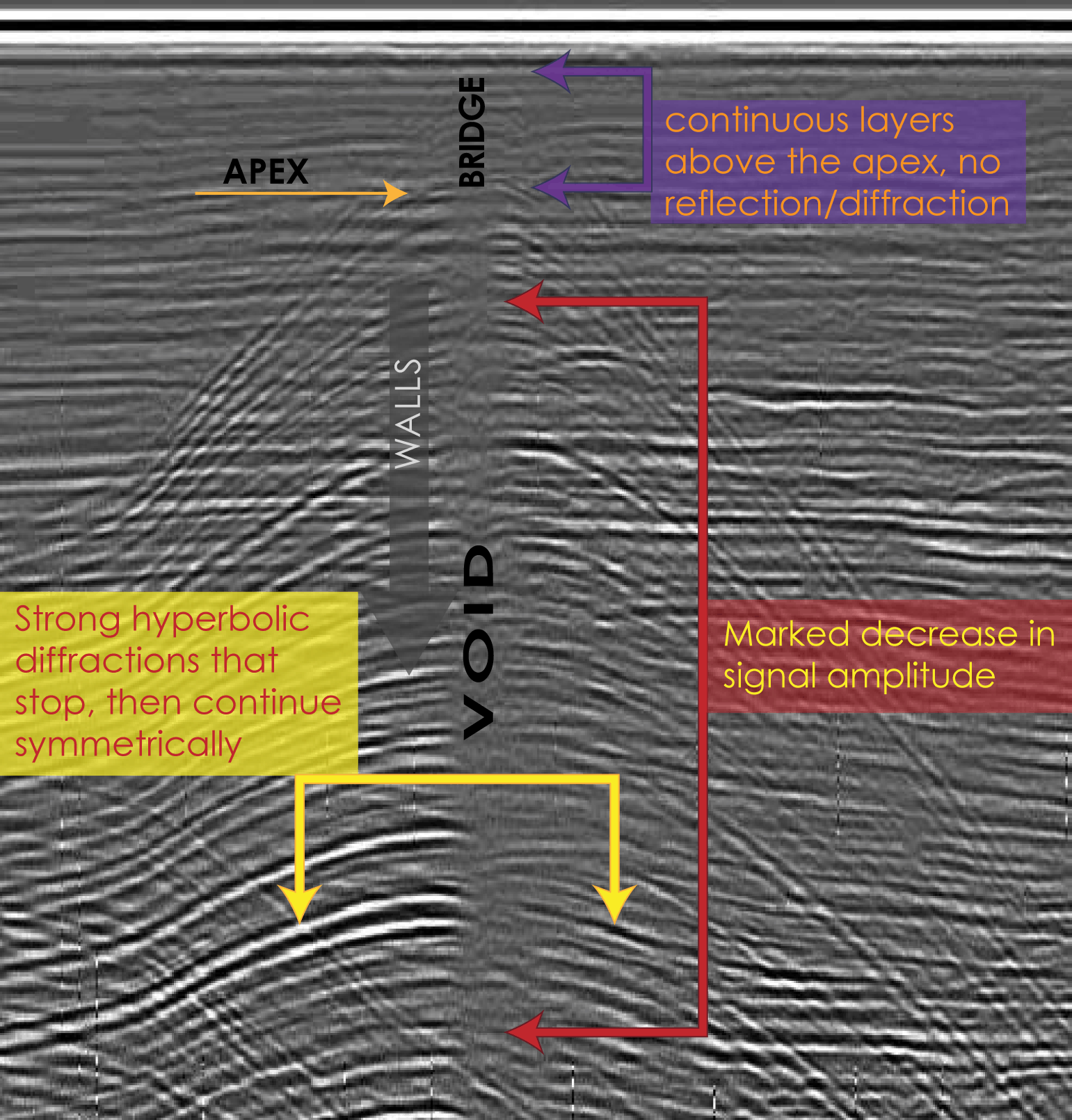
The visual patterns in the data, as previously mentioned, are three-fold: hyperbolic refractions with high power/contrast, The distinction between a region of homogeneously decreased amplitude over the void between the slow undulating, softer reflections of the "background" snow stratigraphy, and the presence of a snow bridge, manifested as a continuance of the undulating reflections directly over the low energy void region. These three features encompass the distinctive characteristics for the field radar operator, and many GPR classification tests are based on attempting to incorporate these patterns as features of a model. A decision to be made must be whether training data will be raw, image based, or physical property based. In the literature review section, efforts will be highlighted from each approach.

Literature Review

Most, if not all machine learning applications to Ground Penetrating Radar data are aimed at detecting and classifying unexploded land mines (UXOs), but this technique could have applications in many other areas, such as archeology, forensic science, meteorology, and geology. There seem to be two trends of approach, namely image characteristic based classification, and physical property based classification. Image properties include edge detection, contrast analysis, texture estimations, and the like. They are based solely on original or enhanced visual features in the image, and similar methods to image classification and characterization can be used [4]. Physical property based classification involves either raw amplitude data as features, or calculated quantities that are meaningful or representative of a part of the data. Though this method may be considered pre-processing, the subjective nature of the pre-processing is minimized if smoothing, averaging, edge/shape enhancement are eschewed or at least used with caution.

There is interesting potential interms of features, or observations that may be useful. Since the most marked visual cue, and the area causing the most grief, is the decreased signal amplitude spanning the length of time the antennae are directly over the void. Specific power, or intensity, of a middle 30cm-wide chunk of the void would be much lower than the other two types of areas encountered. The power distribution is much more dispersed within the hyperbolic regions, whereas it is almost homogeneous within the void. One group [5] uses polynomial curve fitting parameters as features, where the hyperbola apexes are recorded, and points to the right and left of the apex with similar amplitude are used for curve fitting.

Time

Hidden Markov Models would not require a dimension change on the x axis from time to distance, and the number of states need not equal the size of the input vector, where the aforementioned features could be the observables of the states. The model would be able to predict with some amount of certainty, that a certain observable (such as energy density) is resulting from a certain state. The states do not necessarily need to have literal meaning, but it may be inferred based on the corresponding observables present, i.e. a low energy density state may correspond only to a "yes crevasse" state and class label.

A support vector machine based learning scheme for the void is the best use, as individual examples within the void generally do not have a time dependence, and all examples within the void area should have roughly the same features. In the hyperbola region, however, I may have to combine and HMM to capture the importance of the rising hyperbolic, large diffractions. Alternatively, it would be possible to select a small section of this region (~20-30 scans) and look at propagation of the large amplitudes (creating the black hyperbolas) and track the propagation of the peaks, noting their frequency spectrum. As you travel down the x axis of the radargram, it is easy to see that the frequency with respect to depth of "big peaks" increases upon approaching the apex. A wavelet or Fourier transform of high peak signals with respect to depth may be in order.

Preliminary Results

My current dataset contains crevasses from both Greenland and Antarctica, and discussions with pioneer Steve Arcone from CRREL have realized an added data acquisition opportunity: since GPR data is completely scalable by setting the time window and scan rate, small models built with material with similar dielectric properties of snow and ice will produce an additional dataset, very comparable to the real thing. Teflon and plywood, and possibly styrofoam are all media options.

Preliminary results are from a very small training set so far, approximately 300 examples from the void and hyperbola areas. A soft margin SVM classifies one example corresponding to the raw amplitude values, correctly doing so 32 out of 60 times. Considering the input was so high dimensional, and rather uninformative in a time-invariate setting, the classification is adeqate enough to warrant continued exploration in this direction.

Items Left To Do

Final Results

The final algorithms tested are described in detail below, as well as feature extraction rationale and labeling strategies. I then present some results obtained, and relate them to each step aforementioned. Finally, I make suggestions for improvement as well as suggested/planned next steps.

Data Processing

The long-term goal of crevasse detection with Yeti is to perform simple, real-time classification, with minimal subjective processing. The term subjective processing encompases any processing algorithms commorly used in signal and image processing, but that require empirical tuning of certain parameters, i.e. the resulting signal is "subjective" to the processing parameters, and also to the coder. Common, and often useful processing steps include:

Data processing exploration

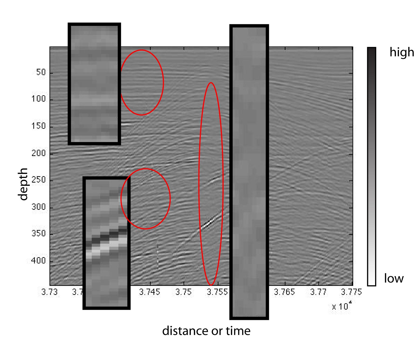
Raw Scan Data

The images commonly shown to represent GPR data are called radargrams. The individual data points are actually 3 dimensional quantities, having depth, distance, and amplitude values. It is convenient to plot distance vs. depth, with amplitude represented as either a RGB or grayscale value, and projected down onto the distance vs. depth plot. This way, it is visually easy to follow white high amplitude spikes for hyperbolic diffractions, as well as a nearly uniform gray area representing the void. A vector of amplitude values corresponding to a constant distance is called a scan, and represents a ** 120-ns** slice of the glacier. Therefore, each scan has "unique" amplitude values, which can be thought of as features of the scan.<\p>

Class labels for each scan are assigned by the author, from field experience identifying crevasses in real time, and discerning characteristic or abberant signatures. The crevasse signatures present at 40 scans per second, and often the first indicator a crevasse might be approaching are the hyperbolic diffractions. With the radar operator vigilant and prepared to hit an emergency kill-switch, he waits until a void is seen, and until a fraction of a second after the symmetric diffractions begin to appear, then stops the vehicle for inspection and marking. This defining sequence of scans is what I use as training and testing data. Each set of training data corresponding to one unique crevasse gets downsampled by 2, resulting in 250 examples of 58-dimensional feature vectors. It has been suggested that downsampling the radargram in this fashion does not significantly change the signature [ref?].

Experiment 1: Train Support Vector Machine with Raw Scans

Experiment 2: Investigate Useful Features of Scans

In other words, the energy is the absolute value of the largest dynamic range of an individual scan. Strictly speaking an energy density measurement would be best (Energy/Area or Volume), but would in effect only weight the current energy by the scan area, taken to be constant. I have not taken into consideration amplitude attenuation at depth, but may need to be considered in the future. This energy calculation makes intuitive sense as a first step, as one of the most prominent but also easy to compute features of a crevasse is the decreased return signal dynamic range. I could also use the average peak-to-peak amplitude instead of the maximum amplitude, and will implement it for the project if I have time.

The downside to the raw scan approach is that taking all scans independently means, if the order of scans corresponding to a crevasse were completely randomized, making visual interpretation impossible, and presented to a trained model, the algorithm would still need to be able to correctly identify a scan "sequence." The word sequence is slightly inaccurate, as time is not being considered at all in the model, but it determines the values of the features as well as the location of patterns present. One of the goals of this project is to determine whether a sequential machine learning algorithm, namely a Hidden Markov Model, is necessary to address this issue of time, or whether a Support Vector Machine applied to chunks of data, possibly overlapping, would be sufficient for real-time classification. The energy calculation seeks to compute an energy curve for an entire crevasse sequence of scans, thereby aggregating all the different depth amplitudes in one scan into a meaningful and informative quantity. The problem is then transformed into one where each example corresponds to an energy curve that represents the changes in amplitude over time/distance. This eliminates the time dimension in the depth(y)-axis, and leaves the time dimension on the distance(x)-axis available if needed.

As expected, computation of energy for each scan of a crevasse signal (which includes the left half of the symmetric diffractions, the entire void, followed by the first 20 or so scans of the diffractions on the other side) results in a characteristic dip in energy at the void, surrounded by higher level energy peaks on each side. This negative spike in energy has two indicative features: peak width and amplitude (recall that this is the peak of the energy over all scans, not of amplitude in one scan). Spike sorting algorithms, which are commonly used for neuron action potential classification in neuroengineering applications, is one option in order to pick out and classify this wide, negative spike in energy. There are several methods common in the literature, including wavelets, FFT-based methods, and polynomial curve fitting. These methods commonly seek to pick out overlapping spikes as well, which is not needed for this application, and therefore these more sophisticated methods are not necessary, and peak width and height should be sufficient information for classification. The peak widths range anywhere from 4 scans to 10. The absolute amplitude is somewhat arbitrary, as the signal suffers from some drift, but the relative amplitude of the spike with respect to the dynamic range is important, as the peak will most likely be near the lower end of the range.

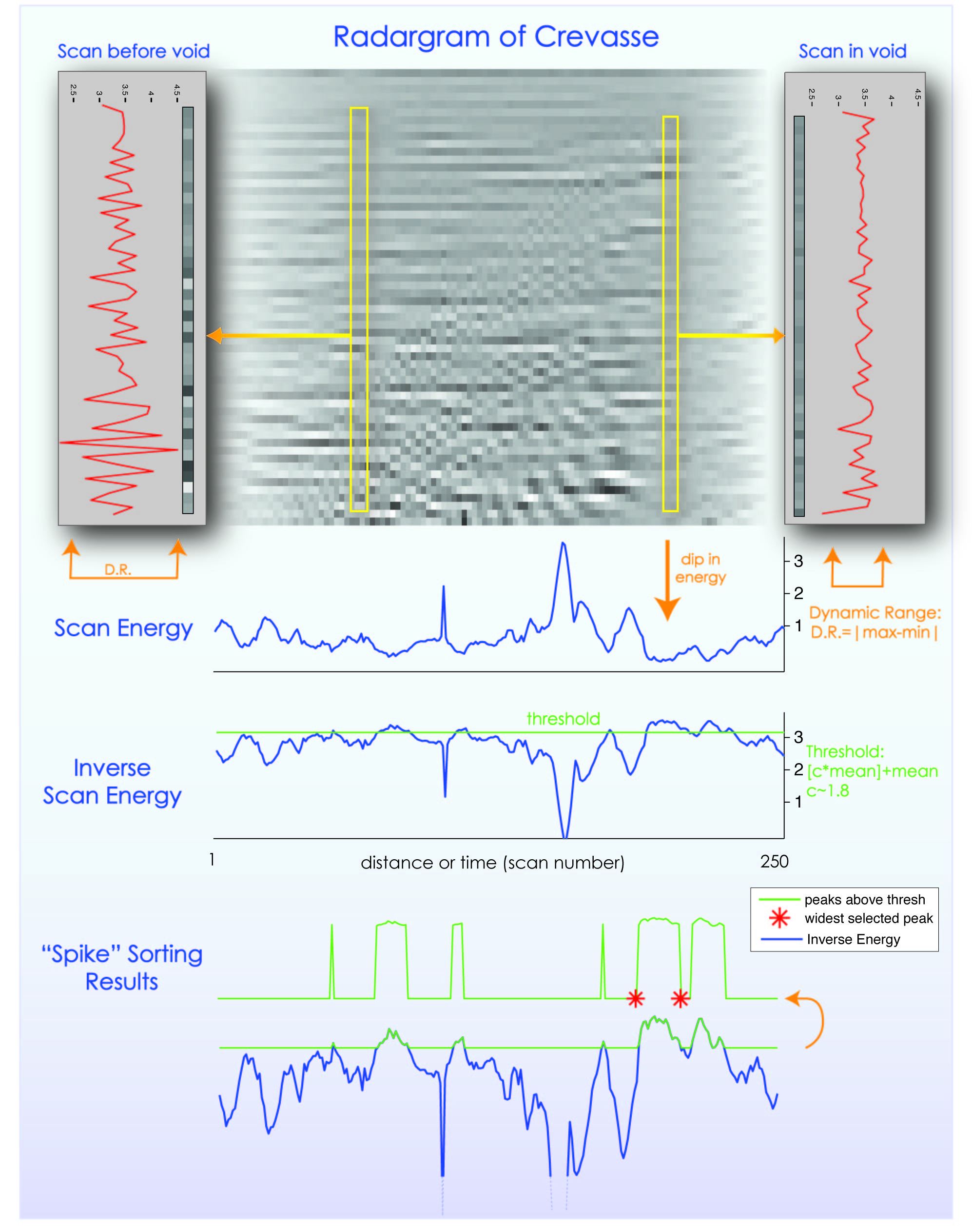
The figure above represents the processing steps and results for the energy spike finding and sorting. I invert the energy signal simply to make computations in terms of positive quantities. The threshold constant, c, I tuned using 5 fold cross validation (by hand), and chose c=1.8.

Results

The total number of examples in existence is ~50 crevasses of 300 scans, comprised of radargrams taken in Antarctica and Greenland in 2010 and 2011. In consultation with literature and references, I have decided that there is simply not enough data to produce a robust HMM. Instead, the final real time algorithm will likely be comprised of two steps: SVM for classifying "crevasse" or "no crevasse" as the scans present themselves, and once a void is detected, the algorithm will look back approximately 200 scans and use them as observations of a 2 state HMM. Therefore, this project will focus solely on the two SVM methods described above, and choose the best and most robust.

The SVM experiment on the raw scan data did well, correctly classifying. The table below summarizes these results.


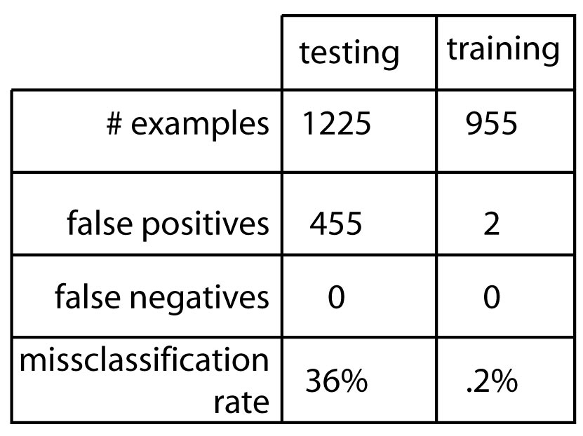
Unfortunately, the classification on Energy data was done in haste, and could not be replicated in time for this report. However, it did significantly worse, and is not ideal since it requires an entire crevasse to train and classify the model, and is not realistic in terms of a real time application. One training session resulted in ~100/660 per spike, where each spike was padded with zeros to be 8 data points long, with 1's labeled where the widest peak was identified. This method does worse because the GPR amplitudes are subject to drift, and it may be that adjacent scan differences in energy are more important than single scan energies. This will be investigated next. Evidently the classifier errs on the safe side, labeling scans as crevasses when there is no void, but never misses a crevasse. A higher false positive rate is much more desirable than a high false negative result, as calling crevasses one is not sure about is better than skipping one. Also, the data were hand labeled, and often a distinction between the diffraction and void areas is gradual on the radargram, and the accuracy of scan labeling is in the range of +/-8 scans, as far as I can distinguish. Crevasses from Antarctica are more distinct than those from Greenland. The next step is to allow padding for the area between the void and diffractions, since hand labeling is subjective, and ground truth measurements are not yet available, and very difficult to get. Real-time classification will simply involve adding each scan to the testing dataset as it is presented, and retesting the SVM in chunks of 5-10 scans.

References

[1] H. Frigui, K.C. Ho, and P. Gader Real-Time Landmine Detection with Ground-Penetrating Radar Using Discriminative and Adaptive Hidden Markov Models, Journal on Advances in Signal Processing, 2005
[2] P.D. Gader and M. Mystkowski, Landmine detection with ground penetrating radar using hidden Markov modelsÂIIEEE Transactions on Geoscience and Remote Sensing,
vol. 39, Jun. 2001, pp. 1231-1244.
[3] E. Pasolli, F. Melgani, M. Donelli, R. Attoui, and M. de Vos, Automatic Detection and Classification of Buried Objects in GPR Images Using Genetic
Algorithms and Support Vector Machines, IEEE International Geoscience and Remote Sensing Symposium, 2008
[4] L.C. Peter Torrione, “Application of texture feature classification methods to landmine & clutter discrimination
in off-lane GPR data,International Geoscience and Remote Sensing Symposium, 2004. pp. 1621-1624.
[5] Q. Zhu and L.M. Collins, Application of Feature Extraction Methods for Landmine Detection Using the Wichmann Niitek
Ground-Penetrating Radar,” IEEE Transactions on Geosc, vol. 43, 2005, pp. 81-85.