Style-based image retrieval and
inference of stylistic classes
Project Milestone
James M. Hughes
COSC 134 - Machine Learning and Statistical Data Analysis
Spring 2011
Recap of Problem Statement
The availability of large collections of digital images via the Internet has necessitated the development of algorithms for searching for and retrieving relevant images, given a particular query [1,2,6]. Traditionally, these algorithms have described images in terms of associated metadata (such as tags), as well as with content-based features and statistical descriptions [3,4,5]. Furthermore, while the digitization of vast archives of cultural artifacts has made these objects more accessible both to the general public and to researchers, the increase in their availability requires more efficient means of locating objects relevant to a particular query [6,7]. Critically, when we consider new classes of images, it may no longer be the case that these images are best described by features related to their content. In the case of works of art, one obvious means of describing these objects is by statistical features derived from their digitized versions. These features could then be used to facilitate a style-based image retrieval system that returns stylistically relevant images with respect to a query image (or query string). I propose a system that implements similarity-based image search using a query image provided by the user, along with the ability to automatically learn the stylistic categories that describe style relationships between images from feedback on search results provided by the system.
Recap of Proposal Goals
Initially, I identified several main project goals, listed below, along with asterisks that indicate which have been completed by the milestone due date:
- Implement the similarity-based image search model*
- Implement the stylistic inference model as described above*
- Validate the model and assess its performance on a set of labeled exemplars*
- Gather data on human usage of the model (in an unsupervised fashion) in order to automatically derive stylistic categories
Progress Summary
Currently, I have collected a large set of images from the internet (using Bing Image Search [2]) and computed a set of features for this set of images (see below), as well as for a number of art images from my own collection. I have implemented the set of similarity functions necessary to compare features from two images in the model. The stylistic inference model itself does not depend on any components that are not already specified (since both the class inference and model learning use the same form). In this sense, I have met my milestone goal of having the recommendation model complete (and thus far have experimented with it), though at present I have not performed any experiments to test the inference capabilities of the model. I have begun supervised tests of the model, and the results of these experiments are described below. I do not anticipate that in the remaining time I will have a chance to test the model on human subjects, so I leave this for future work. Note that, although by the above list it appears I have accomplished all goals I had initially planned to (except for incorporating human feedback), the process of validating the model and assessing its performance is underway but not yet complete. There are a number of more complex and interesting experiments and variations to the model that I believe are worth testing during the time remaining.
Detailed Progress & Results
Image data
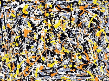
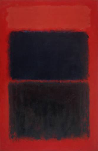
I spent a great deal of time collecting images from Bing Image Search in order to provide some base stylistic classes that could be used to evaluate the efficacy of the model (e.g., I searched for images matching the queries "Abstract art," "Cubism," "Impressionism," and "Renaissance art," among others). Critically, the images returned for each query were stylistically quite diverse, although they did in some sense fit their categorical description. This highlights the fact that stylistic periods are in many ways more historical artifacts than concrete descriptions. For example, the art of Jackson Pollock is quite different from that of Mark Rothko, although both are Abstract Expressionists:
| Pollock | Rothko | |
|
|
|
For this reason, I concentrated on identifying stylistic categories that were more visually consistent. These categories may be individual subsets of an artist's work, separated according to style. For example, I took 79 paintings by Picasso and grouped them according to their common stylistic category. I also created a dataset from drawings by three artists (see below) that have relatively good in-category stylistic similarity. Datasets such as this provide a "simpler" ground truth against which the model can be tested.
Image features
For all the images I considered, I computed eleven different features: [NEED REFS HERE]
- RGB color histograms [8]
- Patch-wise rotational average of Fourier power spectrum [9]
- Patch-wise radial average of Fourier power spectrum [9]
- Basic statistics on patch-wise multiscale Gabor filter coefficients [9]
- Energies of patch-wise multiscale Gabor filter coefficients [9]
- Histogram of line orientations for lines detected using the Hough transform on an edge image [10]
- Basic statistics on line lengths for lines detected using the Hough transform on an edge image [10]
- Patch-wise line density (i.e., number of edge pixels in a patch of fixed size)
- Raw image features (i.e., a downsampled version of each image) [8]
- GIST features [8]
- Slope of the log of the rotational average of the amplitude spectrum [9,11]
Model summary
The learning model is divided into two components, one in which images are recommended to the user according to a target image I and an assumed model of a stylistic class:
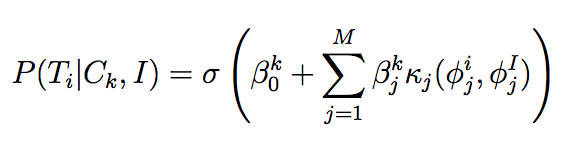
for images T_i in the database and some learned model beta_k, and where sigma is the logistic sigmoid function, kappa_j is the similarity function for the jth feature, and phi_j is the jth feature set for the indicated image. As can be seen, this regression model learns weights according to feature similarities. Once the user provides feedback as to which returned images are relevant to a particular query image I, the system determines the best model according to those responses using
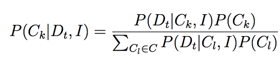
Under the assumption of a uniform prior over stylistic classes beta_k, we can determine the "best" class by choosing the model that best fits user feedback. In essence, each of the beta_k is modeling some stylistic class determined by the user (or users). After a best-fitting model is determined, the model is updated according to user feedback using typical update equations for logistic regression for the model beta_k [12]. Initially, I had anticipated that keeping a moving average of solutions would be the most effective way to update beta_k to take all previously seen information into account, but, as I will describe in detail below, it turns out that this method does not really work in practice (unless the data have very strong in-category homogeneity and strong cross-category heterogeneity with respect to the particular stylistic feature being modeled).
Although I have written my own gradient ascent routine for logistic
regression, I found it to be quite slow in practice, so for my experiments, I am currently using Matlab's
glmfit function, since it is much more efficient than my own. Furthermore, it provides a regularized solution,
which is useful for examining the learned beta_k. If time allows, I will implement my own version of regularized logistic
regression.
As mentioned in the proposal, this model is not useful until it can provide accurate recommendations to users, and this presupposes knowing what stylistic class the user is attempting to model. Barring this knowledge, we could recommend images according to classes already determined (with the possibility of learning new ones later). Thus, we need to "bootstrap" the model by learning some predefined stylistic classes. Most of the initial experiments deal with evaluating the model in this fashion: i.e., can we learn useful stylistic distinctions that are (visually) present in the data in a supervised fashion and leverage this knowledge for the recommendation model?
Experiments
The ultimate goal of this project is to develop a system that is capable of taking user feedback and learning a set of stylistic classes that describes the relationships between images determined by user-provided feedback. However, before this goal can be accomplished, it is necessary to validate the model and to demonstrate that 1) it can learn stylistic distinctions between images described by salient features and 2) that such distinctions actually appear in the data, at least using the features we have at present.
It is critical also to emphasize that the learned models beta_k are not feature-based, but rather feature similarity-based. For this reason, a requirement of model validation is that it is capable of learning the commonalities among similar images according to their features. Since the weights we learn in the logistic regression model directly refer to the individual feature similarities (although the method for calculating these similarities is effectively hidden from the model), we can interpret large (relative) weights as placing strong emphasis on the corresponding feature. This suggests a means to initially validate the model: create images that vary according to a particular stylistic feature (or set of features) and evaluate the degree to which the model is capable of "recognizing" which features are important and which are not.
Experiment 1
To validate the model and demonstrate that it is capable of learning which features are important in a highly controlled setting, I created two sets of random images, each of which contained variation along a particular feature.
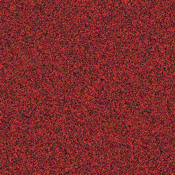
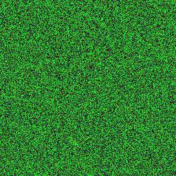
The first set of random images I created were random RGB images that varied according to their color histograms (i.e., "color"
was the perceptually salient dimension of stylistic variation). I created three "stylistically distinct" subsets of random
images by first creating, for each image, three 256x256 pixel uniform random images using Matlab's rand function. Each
of these represented the red, green, and blue channel of the random image, respectively. In order to emphasize one of the three color
components, I multiplied the noise image in either the red, green, or blue channel by a factor of 3. Effectively, this makes images
whose (for example) red component at a particular pixel is on average three times larger than the corresponding green or blue component.
This will cause images to appear more red, green, or blue, depending on the category. I created 75 random images from each category.
Critically, since the images are noise images, they should not meaningfully vary according to any other stylistic feature.
| Example images from each class in color experiment | ||||
| Red image | Green image | Blue image | ||
|
|

|
||
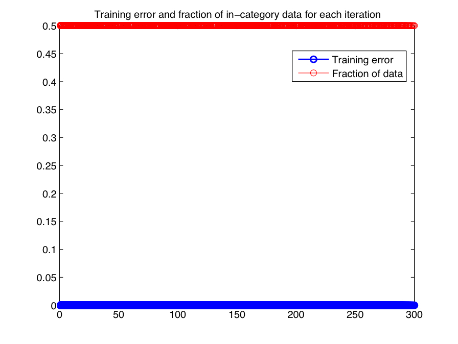
I trained the model in the following fashion: first, I held out 25% of the overall data for testing, and on the remaining 75%, I trained the model over 100 iterations for each category. At each iteration, I took one image at random as the target image and then, based on what category it fell into (in this case, "red," "green," or "blue"), I randomly selected 15 in-category images and 15 out-of-category images and used these as the training set. This effectively models balanced user feedback indicating that some relevant images are in the desired class, and others are not. We can compute training error for each iteration of this experiment (i.e., how well the learned model actually separates the training images). In this particular experiment, we need to learn only one beta_k, since we are only attempting to model one distinction (i.e., color).
For each iteration of the experiment, we call glmfit to learn a set of weights beta for the given similarities between
the target image and the 15 in- and out-of-category images. We store each of these learned models to use for testing. Since we have
three classes, there are 300 overall training iterations. Figure 1-1 displays the training error at each iteration for the learned
beta_k and the training images. The first 100 iterations refer to training on red images, the second 200 on green, etc. Also
plotted in the same figure is the fraction of in-category images per test (in this case always 0.5). As can be seen, the model is able
to accurately predict the class (in- or out-of-category) for all of the training images in each iteration. This is not surprising,
since the images vary strongly between categories (and very little within a category) according to their color distribution.
| Figure 1-1: Training error in color experiment. |
|
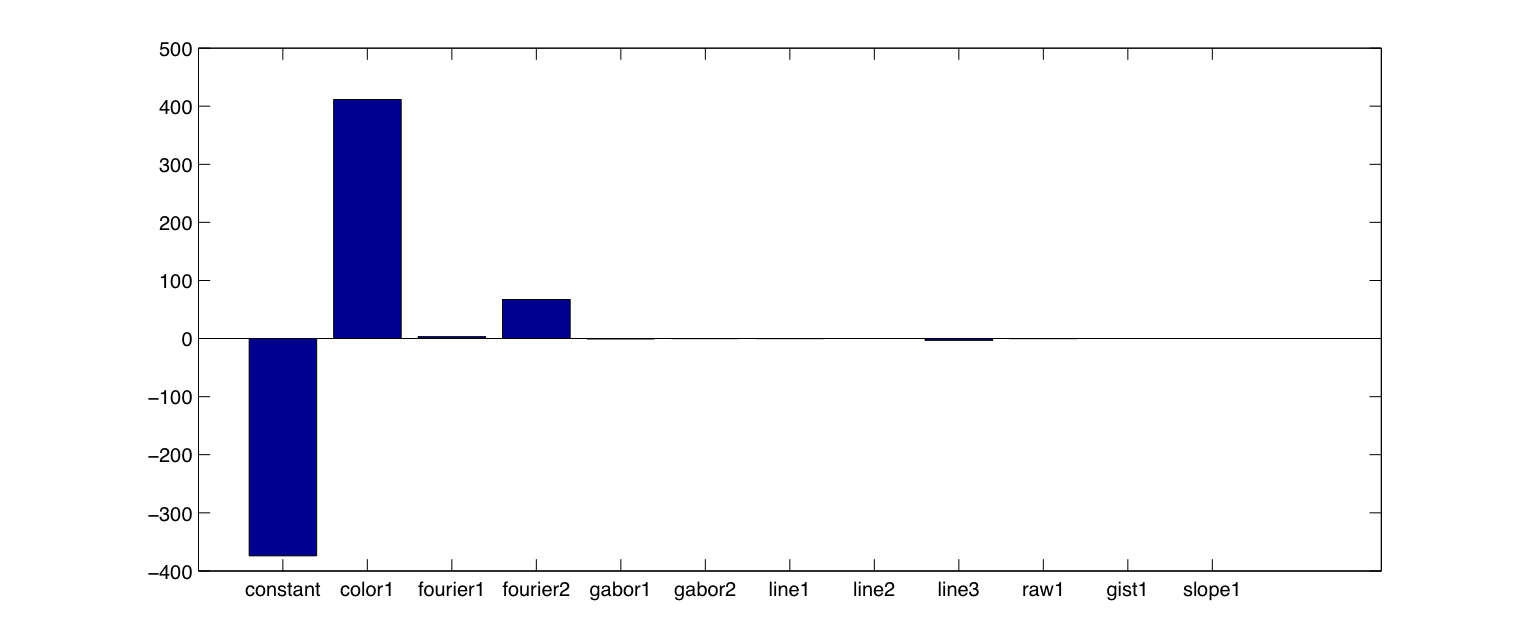
In order to assess the generalization capability of the learned model, it is necessary to determine a single estimate of beta among
all the learned models (since we have a model for each training iteration). Despite having many estimates, because the image categories
vary along a single feature, the learned models should show consistency in the way they emphasize the color feature. A natural way to
select a single beta is to use the mean of the learned betas. Figure 1-2 shows the average of the beta weights
over all training iterations. Although there is a large weight on the constant term, the color feature (color1) shows the
strongest weight of any feature, indicating that it plays an important role in separating the categories of images.
Figure 1-2: Average of betas over all training iterations in color experiment using glmfit.
|
|
During training, glmfit displayed several warnings indicating that the problem was overparameterized (which makes sense,
since only one feature is controlling the categorical distinction; the others should play essentially no role). To verify the results of
glmfit, I also ran the same experiment (with the same training and testing datasets) using my gradient ascent routine.
Figure 1-3 shows the average of the beta weights learned in each training iteration using my routine.
| Figure 1-3: Average of betas over all training iterations in color experiment using gradient ascent. |
|
Using gradient ascent, the color feature clearly dominates. For both learned models (i.e., the average of the betas obtained
with both glmfit and my own routine), I computed the testing error by considering each held-out testing image individually
and predicting the classes of all the remaining test images using the current testing image as the target image. As before, images whose
original category (red, green, blue) matched the current testing image were considered in-category and all others out-of-category. The
testing error rate was taken to be the average of the error rates for each of these experiments. For each model, I obtained an overall
testing error of 0%, indicating that I was able to perfectly predict the categories of the held-out images using each learned model.
Experiment 2
I performed a similar experiment using images that varied according to a different feature, namely the slope of the log rotational average of the amplitude spectrum. Shown below are two images, one noise image with a flat amplitude spectrum, and another whose frequency spectrum has been modulated so that it contains more low-frequency than high-frequency information. This will affect the slope of the line fit to the log of the rotational average of the amplitude spectrum in a consistent way, so this feature should stand out as being important.
| Uniform noise image | Modulated image | |
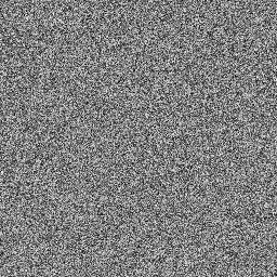
|
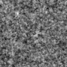
|
|
| Comparison of log rotational average of amplitude spectra for images above. |
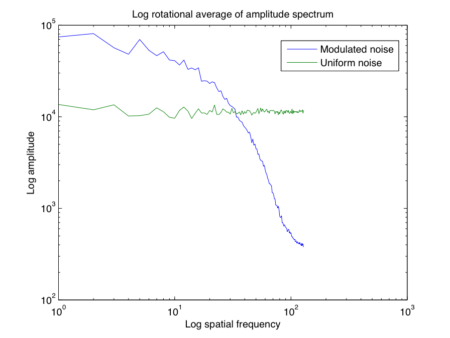
|
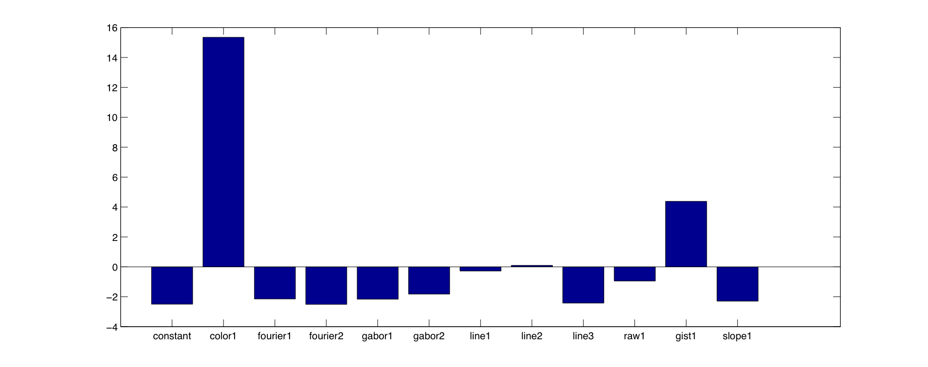
This experiment was run precisely as before, and using the gradient ascent routine and averaging the learned betas in the same way as before, I achieved testing error of 0% overall. Figure 2-1 displays the beta weights used for prediction; the slope feature has the largest coefficient, although others have some (relatively) small values. The GIST feature may have a large positive weight to offset the other negative features, though it is perhaps the case that GIST, which is computing features from a multiscale decomposition, is picking up on the differences in frequency characteristics between images in this experiment as well.
| Figure 2-1: Average of betas over all training iterations in slope experiment using gradient ascent. |
|
Experiment 3
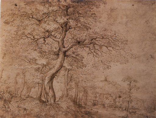
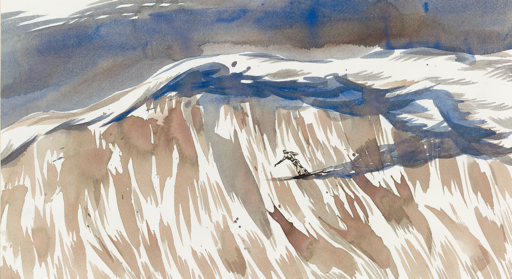
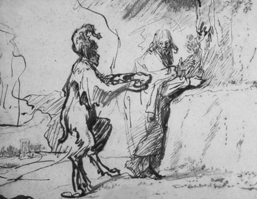
The results demonstrated so far deal with images created in a highly controlled context and thus do not reflect images of the type that would be encountered generally. The goal of this project is provide a platform for style-based image retrieval, so it is natural to consider instead categories of art images that are stylistically consistent. For this experiment, I took several images of drawings from three artists whose drawings are relatively stylistically consistent (though quite different from one another), namely Pieter Bruegel the Elder, Raymond Pettibon, and Rembrandt. The set of Rembrandt drawings also included several by his pupils, though these are certainly more stylistically like the true Rembrandts than they are like the drawings by Pettibon or Rembrandt.
| Example images from each class in drawing experiment | ||||
| Bruegel | Pettibon | Rembrandt | ||
|
|
|
||
As in previous experiments, I held out a fraction of the data (in this case 25%) for testing and trained on the rest, using 100 iterations per image category (Bruegel, Pettibon, Rembrandt) to train a model, choosing a random image from each category as the training image and then using a balanced set of in- and out-of-category exemplars to train the model (e.g., if there were 10 in-category images wrt the current training image, I would also select 10 out-of-category images at random from the training set). Figure 3-1 shows the training error for all iterations, where the first 100 refer to training models for Bruegel drawings, the second 200 for Pettibon drawings, and so on.
| Figure 3-1: Training error over all training iterations in drawing experiment using gradient ascent. |
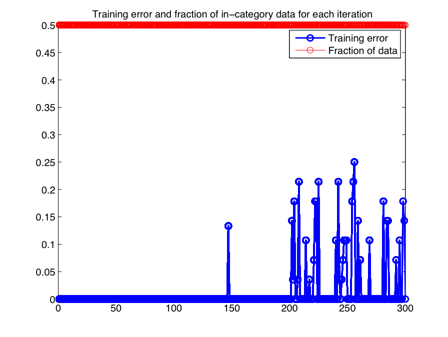
|
As can be seen in Figure 3-1, the training error increases considering in the last 300 iterations, indicating that it was considerably more difficult to separate the Rembrandt drawings from the others. Given the 300 models learned, it is necessary to choose a representative model for each class. Figure 3-2 shows the pairwise correlation distance matrix between all learned betas. The first 100 rows/columns refer to Bruegel, the second 100 to Pettibon, etc.
| Figure 3-2: Pairwise correlation distances between all learned models in drawing experiment. |
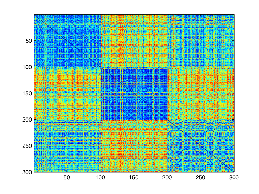
|
This figure indicates a great deal of consistency between the models learned for each target each from each category, suggesting that taking the average of the betas for each category might provide a good representative model for each. Using this strategy, I took the average of all beta weights learned for the Bruegel drawings, Pettibon drawings, and Rembrandt drawings and created three models. Figure 3-3 shows the per-class per-model overall error rate for the testing data. This was computed by considering each held-out testing image as the target image and predicting the class labels of the remaining image wrt this image (where drawings from the same class as the target were considered in-category and all other images were considered out-of-category). Error rates reflect the average over all target images from each class.
| Figure 3-3: Per-class per-model error rates averaged over all testing images. |
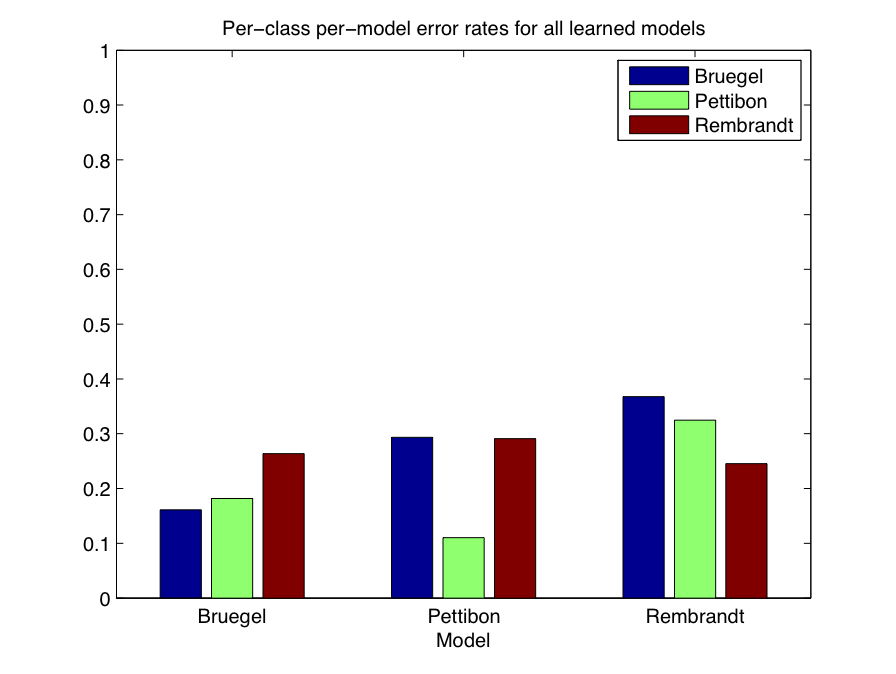
|
It is also instructive to consider the in-category error rate for each model, as well. That is, we will consider the fraction of times that in-category images were incorrectly judged as being out-of-category. In some sense, this is a more useful measure than overall error for two reasons: first, there are often more out-of-category images than in-category images (since in-category refers to a single class of image, and there may be several under consideration); second, in the context of image search, it is in some sense "more important" to return relevant images, even with a few irrelevant images, than to return no irrelevant images, if that means that no relevant images are returned either. Figure 3-4 shows the in-class error rates for each class, for each model. Once again, these represent averages over all target images of a particular class.
| Figure 3-4: Per-class per-model in-category error rates averaged over all testing images. |
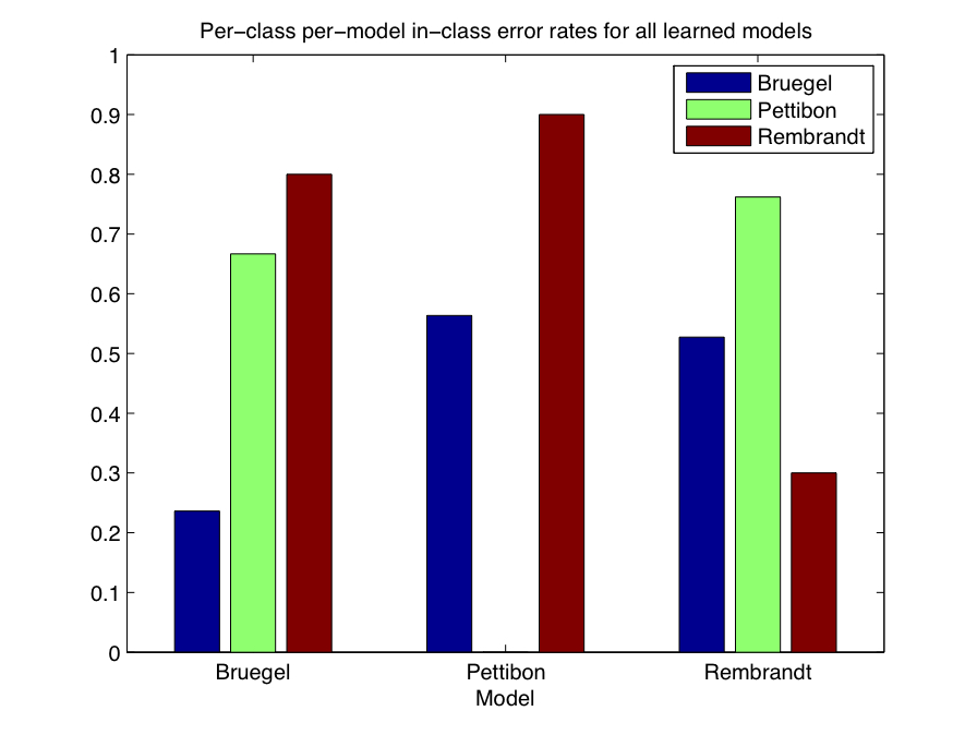
|
Figure 3-4 is particularly instructive, as it shows that, while overall errors are relatively low for all image classes across the three learned models, Bruegel drawings had the lowest in-category error rate for the first model, while Pettibon drawings had the lowest error rate for the second model, and Rembrandt drawings had the lowest in-category error rate for the third model.
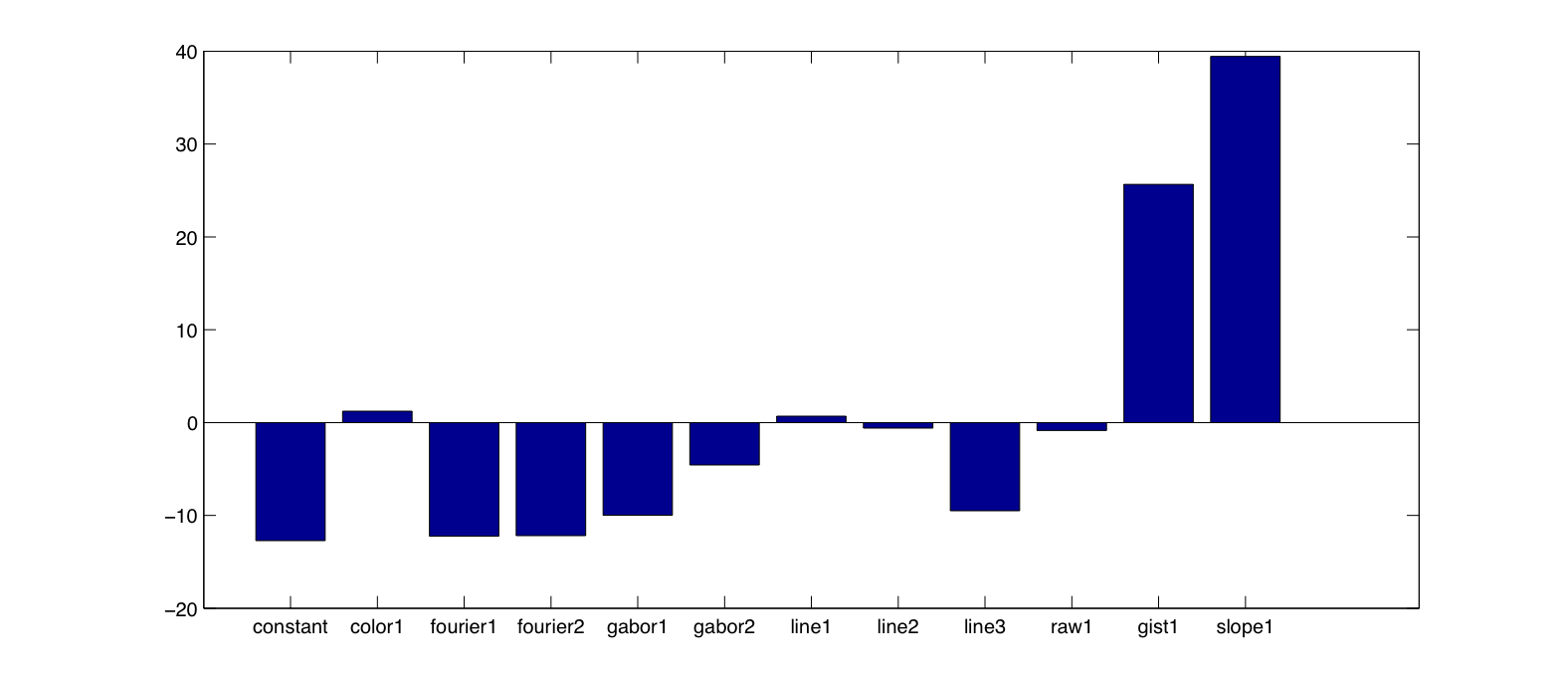
We can also examine the learned models more closely by considering the learned models shown in Figure 3-5, as represented by the way in which they weight each individual feature. Visually, there appears to be more consistency between the Bruegel and Rembrandt models, which is also reflected in the distance matrix shown above.
| Figure 3-5: Learned beta weights for each of the three models. |
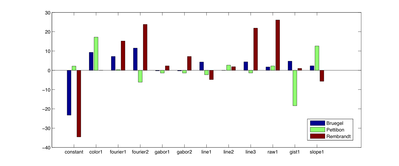
|
I also considered the inferential capability of the model, i.e., treating the in- and out-of-category testing images wrt a target image as simulated feedback, I looked at which model provided the largest log-likelihood of the data. This simulates a model inference step in a real-life setting, and the expected result would be that the best model according to log-likelihood would in fact be the model corresponding to the category of the target image. For example, if the target image is a Bruegel drawing, then we would expect the Bruegel model (averaged over all training iterations) to provide the best fit to the observations. This is another way besides class prediction of evaluating the learned models. For the corresponding models as shown above, I achieved a 26% model inference error using all the testing images (other than the target image, of course) and 0% error considering only in-category images. Obviously this information would not be known in practice, but such a low error rate does demonstrate that the model is capturing some salient characteristics of the images.
Future work and thoughts on progress so far
For the remaining time, I will train the model on more complex problems and also look into examining what recommendations the model makes (after bootstrap learning) in order to provide another means of assessing its validity. If time allows, I may also add more features to my feature set. I also want to concentrate on using the style inference model to automatically determine the relevant stylistic class, using some of the training images as simulated feedback and the testing images as potential recommendations.
One problem I have encountered so far seems to stem from the problem of having many categories of images. During training, the model considers all images from a single category (e.g., Bruegel drawings) to be in-category and all others to be out-of-category. This means that, as the number of image categories grows, it may be increasingly difficult to learn models that separate all of the out-of-category images from the in-category images, even when there is some consistency among the in-category images. I think that perhaps this is a weakness of my model, in that it views pairwise similarities in a local manner. I think the model is strong in that it is learning distinctions that do not depend directly on the features, but in practice it seems that the assumption that there will be a single set of weights that captures the within-class stylistic consistencies and simultaneously perfectly separates the in- and out-of-category data does not hold. In particular, although it may be possible to separate an artist's work from those of all others, multiple models may be needed to capture these distinctions. Also, since the logistic regression model is learning a linear separator in the similarity space, this may account for its inability to separate the in- and out-of-category images effectively. I intend to explore these issues futher in the remaining time, including weighting in-category datapoints more heavily than out-of-category datapoints, since typically there are many more out-of-category exemplars, yet it would be beneficial to consider all of the (training) data when learning a model.
References
- "Google image search," http://www.google.com/images.
- "Bing image search," http://www.bing.com/images.
- N. Vasconcelos, "From pixels to semantic spaces: Advances in content-based image retrieval," IEEE Computer, 2007.
- M. S. Lew, N. Sebe, C. Djeraba, and R. Jain, "Content-based multimedia information retrieval: State of the art and challenges," ACM Transactions on Multimedia Computing, Communication, and Applications, 2006.
- Y. Chen, J. Li, and J. Z. Wang, Machine Learning and statistical modeling approaches to image retrieval. Kluwer Academic Publishers, 2004.
- "Google Art Project," http://www.googleartproject.com/.
- S. Hockey, "The history of humanities computing," in A Companion to Digital Humanities, Blackwell Publishing, 2004.
- C. Wallraven, et al., "Categorizing art: Comparing humans and computers," Computers & Graphics, vol. 33, 2009.
- T. Pouli, D.W. Cunningham, and E. Reinhard, "A survey of image statistics relevant to computer graphics," Computer Graphics Forum, vol. 00, 2011.
- J. Illingworth and J. Kittler, "A survey of the Hough Transform, "Computer vision, graphics, and image processing," 1988.
- D. Graham, J. Friedenberg, D. Rockmore, and D. Field, "Mapping the similarity space of paintings: image statistics and visual perception," Visual Cognition, 2009.
- C. M. Bishop, Pattern Recognition and Machine Learning. Springer, 1st ed., October 2007.