Soft clustering dynamic networks with probabilistic tensor factorizations - Milestone
Nick Foti
Introduction
Network data is ubiquitous with huge amounts being constantly collected in a multitude of application areas. Common analyses of network data treats the observed networks as static snapshots which provides a simple framework to study the network. However, real networks evolve over time and so the underlying dynamics must be taken into account to better understand them.
A common problem in network analysis is clustering the nodes into groups of similar nodes (co-clustering in the case of bipartite networks). Current methods for clustering networks only consider static networks. The only existing way to cluster a dynamic network is to independently cluster static snapshots of the network at each time with a traditional graph clustering algorithm (e.g. spectral clustering) and then post-hoc infer dynamics from those clusterings. This seems unsatisfying, so in this work we propose and implement probabilistic models and inference algorithms to simultaneously infer clusters and the dynamics of the clusters for time-varying networks.
Progress
My progress is just about what I proposed for the milestone. The only point that I would have liked to have finished was having all learning algorithms implemented. I still have a block gradient algorithm to implement for the Poisson model, however, the reason for not having it done is that I didn't think I would need it until very close to the milestone data. That being said I did propose alternative learning algorithms for the Poisson model only if necessary. I believe that this algorithm will not be challenging to implement and I will be right back on track with the rest of the project.
Data
We consider both synthetic and real data to evaluate the effectiveness of the proposed models. The synthetic data is used to validate the learning algorithms and to provide a dynamic network with a "ground truth" clustering to compare our learned clusters to. We consider real data from three application areas described below that represent both the clustering and co-clustering problems.
Synthetic data
We consider two types of synthetic data. The first type is random data generated from the proposed statistical models. These synthetic data are used strictly to test the convergence of the learning algorithms and are not intended to represent meaningful clustering. The proposed models will be described in more detail below. For each model we generate a sparse third-order tensor with a specified number of non-zero entries (or a specified fraction of nonzero entries) per time. The number of latent factors is also specified apriori. We divide the non-zero entries of the random tensor into a training and validation set. As mentioned previously, we then use this data to test the convergence of our learning algorithms.
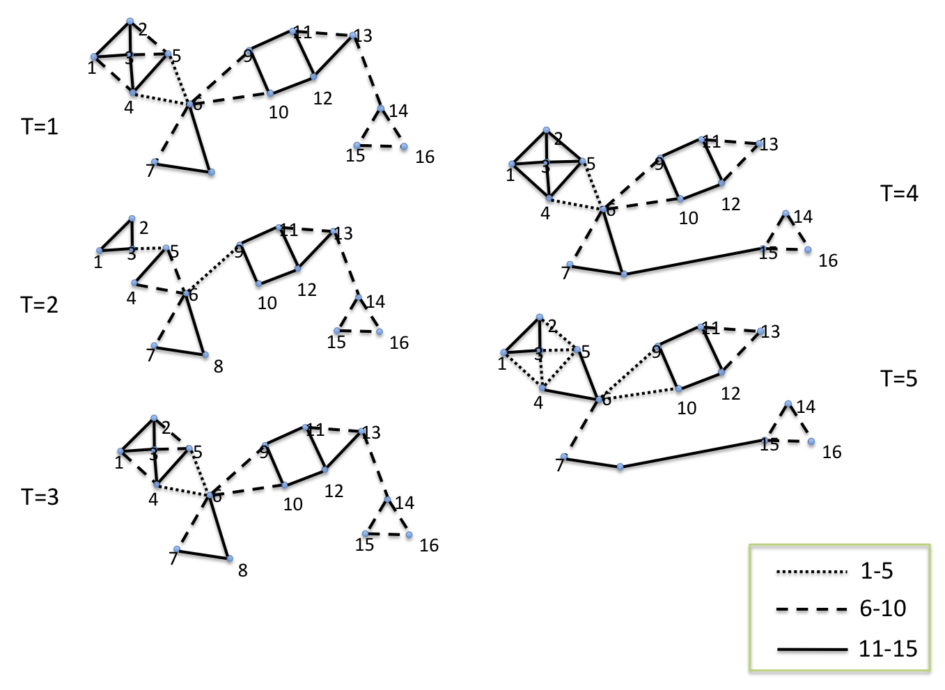
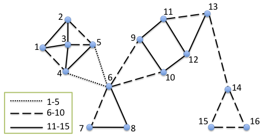
The second type of synthetic data we consider is a small hand-made network that evolves over time with known clusters. The data is snapshots of a 16 node network at five time stamps. Figure 1 depicts the network at the different time stamps. There are obvious clusters at the various time points, some of them constant over time, others going in and out of existence.
Real data
The first real data set we consider is the World Trade Web network. This network contains 196 contains corresponding to countries and directed edges between countries such that an edge from country i to j indicates the amount of U.S. dollars exported from country i to country j. Each edge has an associated time stamp in the years 1948 to 2000. Note that the network is directed and that nodes are not necessarily present at each year. The goal with this network is to find clusters of countries over time and so represents the clustering problem. Table 1. reports some useful statistics of the world trade web network.
The second real data set we consider is the evolving network of correlations between the monthly returns of equities from the S&P 500 stock index from January 2005 to December 2007. These dates were chosen as it produces a manageable size data set and represents a more or less normal period for the market. The data was constructed by obtaining the daily closing prices of the stocks from the S&P 500 using the DataStream service. The prices were converted to returns using the standard formula:
R[i,t] = (P[i,t] - P[i,t-1]) / P[i,t-1]where R[i,t] and P[i,t] are the return and price of asset i at time t, respectively. The time series of returns are then smoothed with a 20-point moving average filter. A month of trading days is roughly 20 days, thus the choice of a window size of 20. We then compute the correlation matrix between equities for each month using the values of the smoothed series for each day of the current month. The hope is that the smoothing performed will mitigate any edge effects introduced by the finite window size. See Table 1 for some overall statistics. This network represents an instance of the clustering problem as the goal is to cluster stocks over time.
The last real data set we consider consists of authors publishing at ACM conferences over time. The data was mined from DBLP and the resulting data is a third-order tensor where the (i,j,l)'th entry contains the number of paper that author i published in conference j in year l. This tensor represents an evolving bipartite network where the goal is to find clusters of authors and conferences simultaneously and so represents the co-clustering problem. See Table 1. for general statistics.
| # Nodes | # timestamps | # Edges | Sparsity | |
|---|---|---|---|---|
| WTW | 196 | 53 | 48336 | 2.37% |
| Equities | 474 | 36 | 28768 | 0.36% |
| DBLP | 655551 (auths), 5121 (confs) | 52 | 2294930 | 1.315e-05% |
Models and learning
We develop two statistical models for the evolving network data considered. The first model posits that edges arise from a Normal distribution and is natural for networks where the observed edges may be positive or negative, for instance if modeling the deviation from a baseline, e.g. ratings. The second model posits that edges arise from a Poisson distribution and so is natural for networks with all positive edges that are integers, e.g. counts.
Normal model
The normal model posits that given factor matrix U (K x M), V (K x N) and W (K x L) that the entries of the third-order tensor X (M x N x L) are generated from a Normal distribution,
X[i,j,l] ~ N(mu,sigma)where mu = sum(U[:,i].*V[:,j].*W[:,l]) and sigma is a constant variance. We place Normal priors on the entries of U and V with mean 0 and variances sigma_U and sigma_V respectively. To model temporal dependence in the factors we make the columns of W follow an AR-1 process,
Intuitively the U and V matrices indicate the degree to which the factors contribute to the connections that the nodes make. The matrix W indicates when factors are active and inactive.W[:,1] ~ N(muW,sigma_W) W[:,l] ~ N(W[:,l-1],sigma_W), l in {2,...,L}
The use of the Normal distribution means that generate edge values may be positive or negative. Most network data is inherently positive so at first glance the Normal model might not seem to be a good idea. One reason to formulate the model is that some network data may be well modeled as a deviation from a baseline. In this case one would first subtract the mean value from all edges and then the Normal distribution is a natural distribution for the deviation (modeling this type of data is not a goal of this work, but it is important to notice). Even in cases where we only observe positive data the Normal model may be useful. Note that there is no constraint the the columns of U, V and W be orthogonal, so when observing all positive data there is nothing keeping the entries of U, V and W from all being positive. In this case we can interpret the learned columns as posterior probabilities of cluster membership and activity.
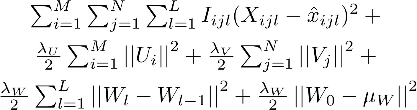
With the generative model specified we can turn our attention to inference in the model. For simplicity we will resort to MAP estimation of the factor matrices U, V and W with the other parameters held fixed. This amounts to minimizing the following error function:
Poisson model
The Poisson model assumes that given factor matrices U, V and W, the edge weights of the third-order tensor X are generated from a Poisson distribution with rate (mean) given as in the normal model. Specifically, we have that
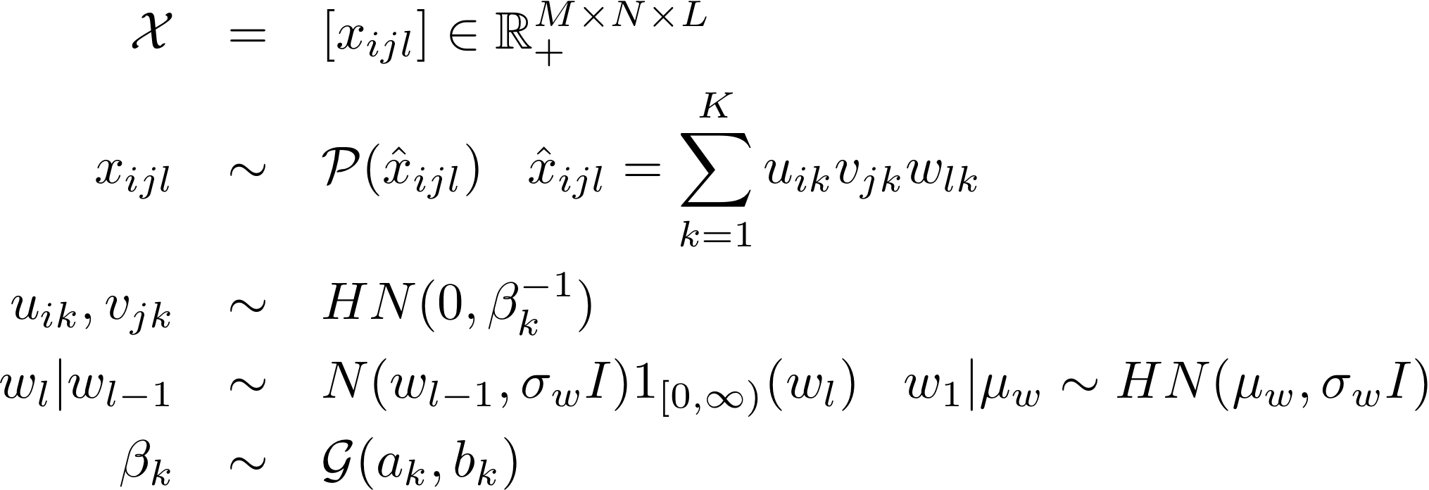
Having specified the generative model we will again resort to MAP estimation of the factor matrices. Our goal is thus to maximize the posterior probability of the factor matrices given the observed tensor. It turns out that the function we are maximizing has close connections with the generalized Kullback-Leibler divergence. We have derived and implemented a stochastic gradient ascent algorithm to learn the MAP factor matrices.
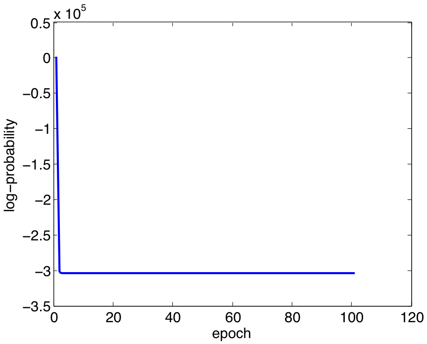
The stochastic gradient algorithm implemented is not very effective at learning a reasonable model as can be seen in Figure 2. This figure shows the value of the objective function for various epochs (number of times through the training data) of the learning. The reason for this is that all beta_k's are being forced to infinity immediately. We have tried to "slow" the first iteration down, however, a block gradient algorithm will be derived and tested. To show
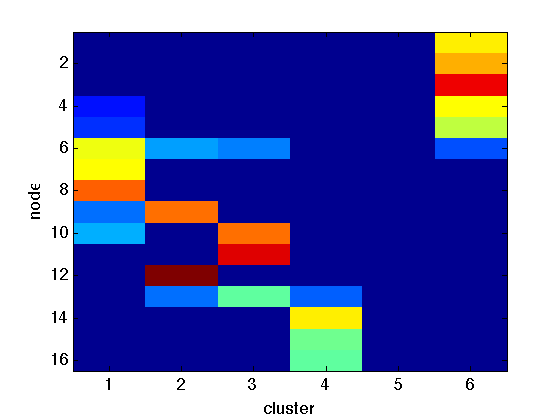
Lastly, we show that the Poisson model does in fact learn good clusterings as well as the number of clusters in the static case. In Figure 3 we show a simple network (the first timestamp of the toy network above) and the indator matrix for the cluster assignments of the nodes. Note that nodes can belong to different clusters with varying weights, and also that the model has learned the number of clusters as cluster 5 isn't used. In this case one cluster does seem to be split into two, but hopefully multiple runs would fix that.
| 
|
Looking ahead
I will have the last learning algorithm I will consider implemented very soon and will then start extensive experiments on the toy and real data I have. There are a number of parameters in the models and learning algorithms and the results do not seem very robust to these values so I expect to spend a lot of my time optimizing these. See the following updated time line for a detailed schedule.
Updated timeline
All dates below are completion dates
- 5/10 - Milestone presentation
- 5/12 - Implement block gradient algorithm for Poisson
- 5/14 - Extensively test both methods on toy network, start on real data
- 5/15-5/20 - Gather results on toy and real networks
- 5/20 - ALL ANALYSIS COMPLETE - Buffer period, start poster
- 5/26 - Print poster
Note: Dates above may be subject to change and certain goals may be shifted forward or backward in time depending on progress.
References
- A.Y. Ng, M.I. Jordan, and Y. Weiss. On spectral clustering: Analysis and an algorithm. In Advances in Neural Information Processing Systems 13, 2001.
- I.S. Dhillon. Co-clustering documents and words using bipartite spectral graph partitioning. In Proceedings of the 7th ACM SIGKDD International Conference on Knowledge Discovery and Data Mining, 2001.
- I. Psorakis, S. Roberts, and B. Sheldon. Soft Partitioning in Networks via Bayesian Non-negative Matrix Factorization. In Workshop "Networks Across Disciplines in Theory and Applications", Neural Information Processing Systems, 2010.
- T.G. Kolda, and B.W. Bader. Tensor Decompositions and Applications. In SIAM Review, 51(3):455-500, September 2009.
- D.M. Dunlavy, T.G. Kolda, and E. Acar. Temporal Link Prediction using Matrix and Tensor Factorizations. In ACM Transactions on Knowledge Discovery from Data, 5(2):Article 10, February 2011.
- L. Xiong, X. Chen, T. Huang, J. Schneider, and J.G. Carbonell. Temporal Collaborative Filtering with Bayesian Probabilistic Tensor Factorization. In Proceedings of SIAM Data Mining, 2010.
- V.Y.F. Tan, and C. Fevotte. Automatic Relevance Determination in Nonnegative Matrix Factorization. SPARS 2009.
- A. Globerson, G. Chechik, F. Pereira, and Naftali Tishby. Euclidean Embedding of Co-occurrence Data. In JMLR 8, 2007.
- N.J. Foti, J.M. Hughes, and D.N. Rockmore. Nonparametric sparsification of complex multiscale networks. In PLoS ONE, 6(2), 10, 2011.