Discriminative Random Fields for Aerial Structure Detection
Daniel Denton and Jesse Selover
Project
We chose to work on a computer vision problem: labeling regions of an image depending on the presence or absence of man-made structures. We hoped to replicate the results of Kumar and Hebert [5], who applied a novel model to the problem that they called Discriminative Random Fields (DRFs). Our interest largely derived from our desire to code this algorithm, but the problem of detecting man-made structures in computer vision is important in its own right. Successful computer analysis of images to detect buildings and other man-made structures is useful for classification, retrieval, surveillance, and other applications [6].
In particular, we chose to use aerial photos in our project, rather than the stock ground-level photos used by Kumar and Hebert. Structure detection from the air can be especially important for military and law enforcement surveillance, search and rescue, disaster relief, or even estimating building density statistics that can be used for calculations relating to urban sprawl. Working with aerial photos has the added benefit of standardizing our input images and making the problem slightly easier. Orthophotos are aerial photos geometrically corrected so that the scale is uniform, and perspective effects due to the distance to the camera have been removed [11]. The camera position in these photos also means that lines in man-made structures typically meet at right angles, which are favored by the detection features Kumar and Hebert used [6]. These attributes would seem to make them ideal to study. Due to their importance for applications like mapping and zoning, there is a plethora of high-quality orthophotos available online. Thus, we had little trouble finding data sources which would suit our needs.
Aerial Orthophoto Dataset
We were fortunate to find a public online archive of high-quality orthophotos of the entirety of Montgomery County, Maryland at the Montgomery County GIS website [8]. We selected three-hundred of images from this archive from which to create our aerial orthophoto dataset.
We decided to crop our images to 256x256 pixels split into 256 16x16 pixel sites (the same site size used by Kumar and Hebert [6]). Since the original images we acquired from the Montgomery County GIS website [8] were larger than this, we used a script to randomly crop each image to the desired size. We also had the same script randomly rotate each of our images, because we are interested in performing structure detection which is not dependent on compass orientation.
Since we needed to label 16x16=256 sites for each image, and we intend to label 300 of our own images along with some images from the datasets of previous researchers, it was imperative that we create a tool which simplifies and speeds up the process of creating and storing site labelings. We decided to use python for our data labeling program, because the pygame library provides such great tools for easily creating a simple point and click application.
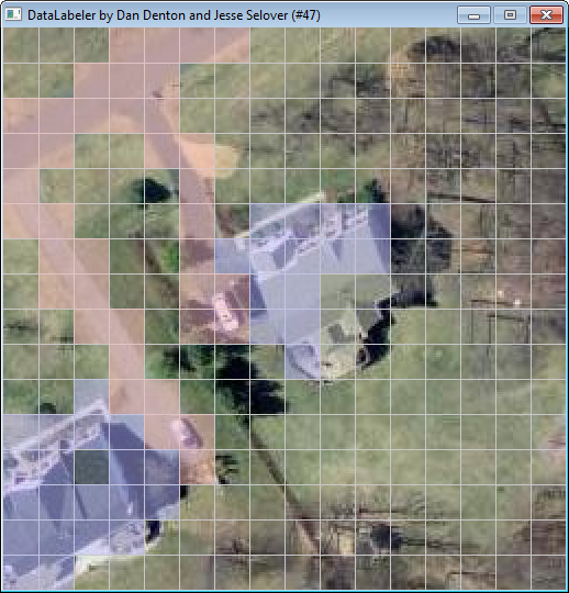
The data labeler continuously backs up the current labeling of each image as a comma separated text file which we then read in our C# implementation. This allows the data labeler to load the latest labeling of any image. By outputting our inferred classifications of test images to this format, we gain the added benefit of using the same data labeler to display our classification results.
Kumar-Hebert Dataset
In addition to trying to classify the sites in our own dataset, we wanted to perform site-classifications on the images that Kumar and Hebert used so that we could compare results.
Shortly before the Milestone, we contacted Sanjiv Kumar who kindly provided us with a copy of the 237 image set that he and Hebert used for their man-made structure detection implementation. This dataset consists of 108 training images and 129 test images, all drawn from the Corel photo database. Each image in this set has one axis with a length of 384 pixels and another axis with a length of 256 pixels, though some of the images were in landscape orientation, and some were in portrait orientation.
Along with each image, Kumar and Hebert had stored their site labelings as pairs of 24 by 16 pixel black and white tiff images. One of the label images uses white pixels to label sites that contain "edgy structure" sections. The other label image corresponding to the same photo stores labels for sites that contain "smooth structure" sections. According to the supplied documentation, for the man-made structure detection task, Kumar and Hebert combined these two labels into a single boolean structure label using a logical or operation.
We wrote some single time execution scripts (saved in KumarAndHebertLabelConverter/) to load each of the tiff labeling files provided by Kumar and Hebert, perform the desired combination, and then save the output as a comma-separated-values labeling file of the type that we have been using with our algorithm implementation. After reflecting each of the portrait orientation images to landscape orientation, and then modifying our DRF implementation and DataLabeler to accept images with 24x16 sites, we were able to train our DRF model on Kumar and Sanjivs data.
We should note that we had hoped to acquire and test on a third dataset used by Bellman and Shortis [1] for a different approach to aerial structure detection. Because we kept working on trying to improve our classification on the K-H Dataset to reach acceptable accuracy levels, we never made it to that point.
Hyperparameters of the Model
We had to make many choices in our implementation of the DRF model. Broadly speaking, we had to choose what features were important, choose hyperparameters for training, and choose an inference method. In choosing an inference method, our hand was somewhat forced, but we had plenty of other choices:
Features
The features we could use are limitless, but to replicate the results of [6], we used the same types of feature. However, this left open many questions about which features presented would work best with our data.
Everything in [6] starts from a gradient calculation. For every pixel of the image, the smoothed gradient vector at that pixel is calculated by convolving with a gradient of a gaussian filter. Then the other features are calculated from this pixelwise information.
The features presented in [6] are multi-scale; first we will explain the features within each scale.
At a given scale, the pixels within each window are grouped together. Their respective gradients are binned into a histogram indexed by orientation, weighted by magnitude. Then, from this histogram, three types of features are calculated:
- Angularity features, which are implemented as moments of the histogram.
- A right-angle-finding feature, which is implemented by finding the peaks of the histogram and measuring the difference between them.
- An orientation feature, measuring the absolute verticality of the gradients in the group.
For our dataset, the third feature type was inconceivable. The justification for that feature was that pictures of structures are taken with upright cameras, but our data was aerial. It could have conceivably been taken from any angle; we weren't sure if it was initially North-South aligned, we didn't know if buildings tended to be North-South aligned, and to top it off we preprocessed our data by randomly rotating it.
We chose to use the first three central-shift moments, as described in [6], as higher moments were so heavily correlated. We also used two inter-scale features as described in Kumar and Hebert's paper, based on the relative angles of the peaks of the histogram between scales.
We also had to choose between the different methods of cross-feature calculation, and between linear and quadratic basis functions for the association features. We ended up using linear basis functions because quadratic ones did not seem to offer significant benefits, and linear functions were much easier to train. We chose to concatenate the two feature vectors to calculate cross-site features, after determining experimentally that calculating componentwise differences to try to learn some sort of linear scaled distance function produced much worse results.
Initially, we had only one scale, but we found, as Kumar and Hebert did, that results were significantly improved with 3.
We briefly considered using three RGB features per scale, in our mad dash to get better features, which would measure the average intensity of each RGB component over the window at the given scale, but the features were ultimately not useful.
We chose, as we mentioned in the milestone, a gradient-of-gaussian filter with variance 0.5, on recommendation via personal correspondence with Kumar and Hebert.
We had to select the method of smoothing on the histogram of oriented gradients; we ended up using a triangular kernel, but since smoothing was restricted to adjacent bins and we chose our bandwidth carefully, it was equivalent to the gaussian kernel used by Kumar and Hebert.
Parameters for Training
We had to choose a variance for the Gaussian prior on the inter-site parameters; via cross-validation on the powers of ten, we eventually selected 10^(-4).
We also chose our convergence criterion based on the function we were trying to optimize; we terminated the gradient ascent when the likelihood only increased by 1 or less. We initially tried a step-length-based method of checking for convergence, but the likelihood criterion was much more invariant under changing the length of our feature vector, which we frequently did.
Investigating our Features
In trying to determine why our logistic classifier was behaving so mediocrely even on Kumar and Hebert's dataset, we suspected our features. We decided to examine the dot product of the parameter vector w together with a site feature set to determine the contributions of the various features to the association potential. We were immediately struck by how incomparable these contributions were.
Among our intrascale features, the contribution (to the dot product of w with the features) from the second moment feature was on the order of 10^1 to 10^3. By comparison, all the other features tended to have contributions of 10^-6 or less. This included the 0th and 1st moments, as well as the right-angle detection feature.
The fact that the second moment feature dwarfed the contributions of the other two moments is really no surprise. This was partially reflected by Kumar and Hebert's decision to drop the 1st moment from their intrascale feature vector. Nevertheless, we would definitely have hoped to find an important contribution from the right-angle detection term. The fact that this term was being completely ignored was very upsetting.
We set out to try to modify our right-angle detection feature so that it would be more useful for the classification problem. Our initial implementation began with the smoothed histogram of gradients, identified the two highest peaks, and then returned the absolute value of the difference between the angles of these two peaks. (Note that this is exactly the approach described by the Kumar and Hebert.)
We printed out the peak information for certain sites, and then compared this to a visual inspection of the corresponding site on the image. One thing that we quickly noticed was that, for many sites containing a strong line the two highest peaks would form a straight angle (and thus the sin of their angle would be zero). This was occurring even in the presence of a strong right angle line if that line happened to be slightly less strong.
This observation prompted us to redesign the right-angle detection feature as follows. We identify the k largest peaks of the histogram (initially with k = 3). We then compute the absolute value of the sin of the angle between each pair of peaks, and return the maximum of these. Thus we are guaranteed to return a large (close to one) value if there is an angle of approximately 90 degrees between any of the k most prominent edge directions.
The new right-angle feature gave a slight improvement of the detection rate, but the trained model still decides that it is unimportant compared to the second order moment. After our presentation on the 29th, Torresani suggested that we try removing the second order moment feature to see how this affected the the learned model. Since the second and first order moments are so closely tied together, we had already decided to follow the lead of Kumar and Hebert in using only the second order moment in lieu of the pair of moments. Therefore, we next tried training with just two intrascale features, the zeroth order moment and the right angle feature for k=3, along with the the two orientation based interscale features. Including all three scales, this gave us a feature vector of dimension eight.
Examining the contributions of the features from this new model, we found that the right-angle feature was still passed over. Instead, the new model relied primarily on the zeroth order moment. Not surprisingly, a logistic model based primarily on the average pixel magnitudes did not provide good classification results.
In order to finally isolate the right-angle feature, we tried removing all of the intrascale moment features and training with just the right-angle and orientation based interscale features, for a total of five features.
The logistic classifier then classified entirely zeros. In conclusion, our right-angle feature is completely useless.
Results on Dataset (our aerial photo dataset)
When we ran our algorithm on our aerial photo data, we got results that were worse than chance. Most of the images were entirely classified as on, with small gaps. We did, however, much better on Kumar and Hebert's dataset; we suspect this is due to faults in ours. The low resolution of the images, and perhaps the percentage of images that were misleading to the model, must have made it hard to do very well.Results on DatasetKH
Our attempt to replicate most closely the hyperparameter choice of Kumar and Hebert gave results that were nowhere near comparable to theirs. They were, however, significantly better than random chance. We used ICM inference, rather than MAP inference, for the reasons we mention, and in aggregate we had a detection rate of 34% with an average of 83 false positives per image. Random chance would give 115. Out of 91008 sites, we predicted 23,674 as on, 19,683 of which were false positives; the number of sites actually on was 11,575. The classifications showed wide variation; some were accurate and interpretable, while others labeled vast swathes of the images as on for seemingly no reason. We speculate that this behavior was partially due to the choice of ICM as an inference mechanism, but if we compare our logistic classifications to theirs, we see that the problem must really lie with our features. They achieved much better results with just a logistic classification than we were able to; either we are training our model wrong, or our features are just not usefully correlated with being a manmade structure. The results we have gotten when removing the moment-based features, and the dependencies we have observed of our model on the moment-based features both indicate that our right-angle detection and orientation-based inter-scale features are effectively useless.
When we tweaked some features and hyperparameters around (we used only the zeroth and second order moments, and changed our right angle feature to be an improvement on theirs), we achieved, on the test set, a detection rate of 13.1% with 14 false positives per image on average. Random classification would have given 43.9 false positives for that detection rate. This is compared to the detection rate of 70.5% with 1.37 false positives per image which was supposedly achieved in [6].
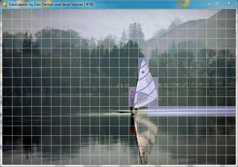
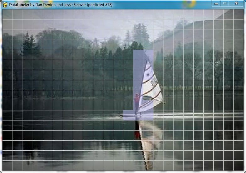
It is also worth noting that some aspects of the the labelings provided by Kumar and Hebert seem subjective. For example, many of there images have sections which we believe to be structure sites which are unclassified, and these sections tend to correspond to sections which are poorly lit, don't have noticeable edgy structure, or otherwise seem like they would be unlikely to work well with the classification algorithm. Alternately, some images have edgy sites which we believe are not man-made structures, but which Kumar and Hebert labeled as such. For example, in the following image (from Kumar and Hebert's training set), the wake of the windsurfer is labeled.
Conclusion
Careful examination of the behavior of our features has revealed that they simply aren't very good. This is especially true for the images in our aerial dataset, where the image resolutions are somewhat varied.
We tried several varieties of features, which included the following itrascale features at three scales:
- the Oth through 2nd order moments
- the right-angle detection features (for the k top peaks)
- the vertical orientation feature
- rgb features
While we have combed through our feature calculation code to see where we could be miscalculating these features, we haven't succeeded in finding where our mistakes lie. Without improving on the features, our classification results are limited to being poor overall. On the K-H dataset, there is a large number of images which are decently classified when using ICM. The logistic classifications, however, are very poor (correlating with the idea that the features are bad). Even with the ICM classification, there are also a large number of images whose classification failed catastrophically, so that statistically the overall performance was marginal.
References
- C. Bellman and M. Shortis. A machine learning approach to build- ing recognition in aerial photographs. In International Archives of the Photogrammetry, Remote Sensing and Spatial Information Sciences, pages 50-54, 2002.
- R. Cipolla, S. Battiato, and G.M. Farinella. Computer Vision: Detection, Recognition and Reconstruction. Studies in Computational Intelligence. Springer, 2010.
- C. Fox and G. Nicholls. Exact map states and expectations from perfect sampling: Greig, porteous and seheult revisited. In Proceedings MaxEnt 2000 Twentieth International Workshop on Bayesian Inference and Maximum Entropy Methods in Science and Engineering CNRS, May 2000.
- D. Greig, B. Porteous, and A. Seheult. Exact maximum a posteriori estimation for binary images. Journal of the Royal Statistical Society, 51:271-279, 1989.
- S. Kumar and M. Hebert. Discriminative random fields: a discriminative framework for contextual interaction in classification. In Computer Vision, 2003. Proceedings. Ninth IEEE International Conference on, pages 1150 -1157 vol.2, Oct. 2003.
- S. Kumar and M. Hebert. Discriminative random fields. International Journal of Computer Vision, 68(2):179-202, 2006.
- J. Lafferty, A. McCallum, and F. Pereira. Conditional random fields: Probabilistic models for segmenting and labeling sequence data. In C. Brodley and A. Danyluk, editors, ICML, pages 282-289. Morgan Kaufmann, 2001.
- Maryland GIS Montgomery County, April 2012.
- F. Shi, Y. Xi, X. Li, and Y. Duan. Rooftop detection and 3d building modeling from aerial images. In Advances in Visual Computing, volume 5876 of Lecture Notes in Computer Science, pages 817-826. Springer Berlin / Heidelberg, 2009.
- R. Szeliski. Computer Vision: Algorithms and Applications. Texts in Computer Science. Springer, 2010.
- various. Wikipedia: Orthophoto, April 2012