Unsupervised Learning of Fundamental Music Features
Richard Lange
Experiments and Results
The conclusion of my milestone presentation was that ISC was working, but the results were ugly and I needed to still tune hyperparameters. I also had not yet looked into PCA yet. A large barrier to PCA (and to ISC, slightly) was that my training images were randomly sampled windows from songs - a major chord would look different based on translations, etc. To address this, I changed the training-data-selection process to only select samples from songs with nonzero values in the first index (top-left corner). Other algorithms that I had considered implementing (i.e. convolutional sparse coding [2]) try to address translation invariance through the algorithm. By more carefully selecting the training data, I avoided having to deal with this.
Test on gratings
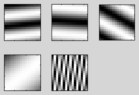
This is the default test in test_iterative_sparse_coding.m. It first generates 5 gratings (oriented sinusoids) and takes a linear combination of them with random weights to generate 25 training images. The weights for this linear combination are taken from an exponential distribution weighted towards zero (so that the best reconstruction could also be sparse).
I used this test to tune the hyperparameters and until the learned features were relatively smooth and seemed to have some semantic meaning. The best results I got by tuning the parameters by hand was with =12 and =100. Larger seemed to make iterations faster. This makes sense given my choice of denseness function: . This function is steep around x=[-2,2]. Updating alpha depends on the derivative of S, so steeper gradient will update faster. Large pulls x closer to 0.
After these tests, I found in the fine print of Olshausen and Field's paper that they set to the variance of the training images and then set to about 0.14*. This was encouraging to find that their / ratio was approximately the same as the one I discovered through testing (0.14 vs 0.12).
RESULTS
5 original features used to construct train images:
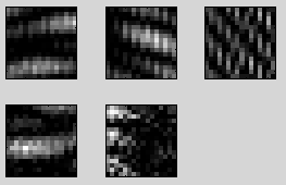
Features learned by ISC, and reconstruction:
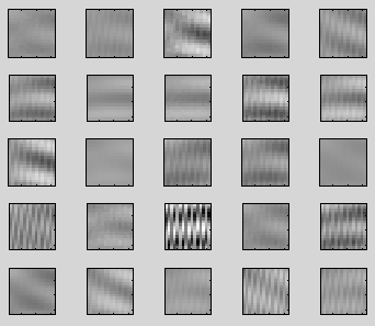
Features learned by PCA, and reconstruction:
Comparing ISC to PCA:
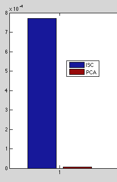
Reconstruction Error
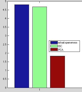
Sparseness of Reconstruction Weights
These results make sense: having learned 5 features, PCA can almost exactly reconstruct the input but doesn't care about sparseness. ISC had slightly worse reconstruction but satisfied the sparseness criteria.
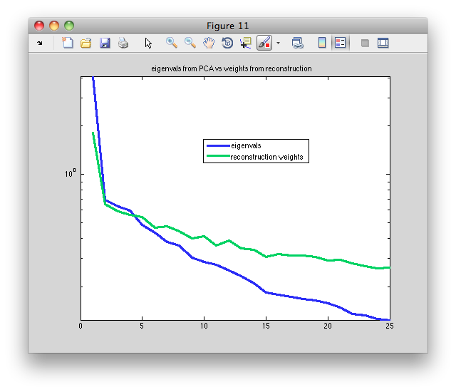
I also compared the eigenvalues from PCA to the weights from reconstruction. They are highly correlated (see image below). This suggests that a good way to compare the features from ISC and PCA is to sort them by corresponding average reconstruction weight or eigenvalue.
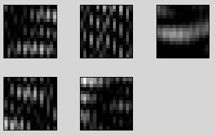
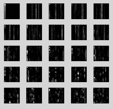
ISC run on music (Joplin and Chopin)
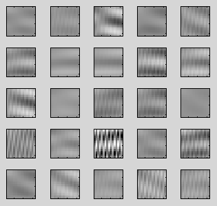
This test (and the next one) looked at 25 songs (18 from Joplin, 7 from Chopin), and sampled windows from each. I took a total of 399 samples, each 12x12 (all with a note in the top left corner to help translation invariance). I had ISC learn 25 features. I tried various combinations of lambda and sigma on this data. The semantically best features came from lambda=12, sigma=100. I also ran trials with the sigma and lambda suggested in [1] (sigma as mean variance of training images and lambda as 0.14*sigma), but these results didn't converge after 16000 iterations (well, the error function was still had a large negative derivative). The following results are from the former test.
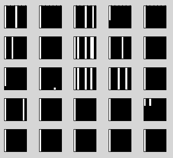
First 25 training images:
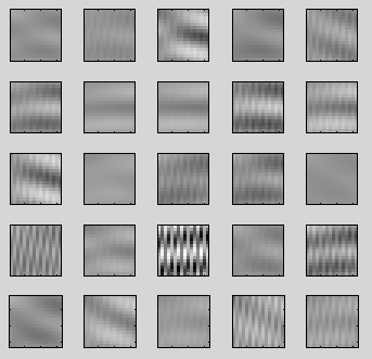
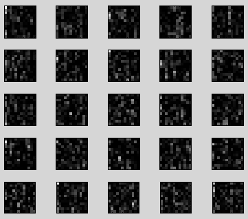
Learned ISC features (sorted by mean absolute value of reconstruction weights, descending) and example reconstruction
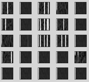
PCA run on various composers
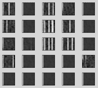
Learned PCA features (sorted by eigenvalue, descending) and example reconstruction
What do these mean?
The x-axis corresponds to pitch. The y-axis corresponds to beat (i.e. a white column is a held note). For the sake of simplicity (and to highlight the translation invariance), assume the left column is C.
the first (most important) feature in both ISC and PCA is a strong first-index, which makes sense because this is the only guaranteed common pixel among all train images
ISC:
The second feature in ISC has faint D, A, and B. This makes less sense, but I also squared each element in these images to make it more readable so high intensity might be negative. In other words, this could be a feature describing "strong presence of D and A and lack of B"..
The third ISC feature seems to be an E, F, and G present in a beat soon after the original C.
The 5th ISC feature is a clear 4th interval.
PCA features make more sense:
feature 2: E, G, A (C-major + 6th or A-minor 7th chord)
feature 3: C, F, A (F major chord, 1st inversion), with slight delay on the F and A
significantly, the 5th feature for both is a strong 4th interval.
To summarize: the features for both can be interpreted, but PCA is much easier.
Classification
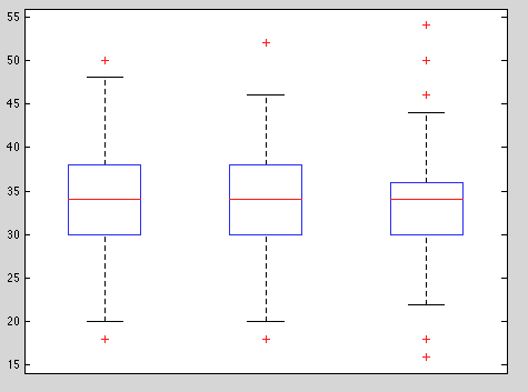
This is a significant addition since the poster presentation. I realized that I did not need to classify full songs, and could instead classify "subsongs" by composer. I implemented this using knn classification with k=3. Unfortunately, I didn't have time to fully test this (though it should be easy). These results should be taken as "preliminary" at best and maybe "buggy." The following test used the same data presented above (Joplin vs. Chopin). The classification feature vectors were computed by convolving the learned song-features from each method with sub-sections of the 25 songs (each 100 beats x all 88 notes). This resulted in a double value for each feature at each nonzero location in the song. For each feature, I then took the mean and central moments (thanks to Jesse Selover) of each feature across all locations in the song.
I used three sets of song-features: one from ISC results, one from PCA results, and one of randomly generated features. Random features provide a good baseline benchmark. As noted in [3], they are a good measure of the classifying capabilities of the model (in this case KNN) independent of the features. I ran 1000 tests which each selected a random 30% of the train set to be used as test-set (hacked n-fold cross validation). The errors were so varied that they are best represented in this box-whisker plot of classification error vs song-feature type:
ISC
PCA
random
The results? ISC performed slightly better than PCA, which was slightly better than random. In fact, the differences were so slight that I would call this result inconclusive.
Conclusions
Ultimately, I never saw the results I hoped to see. I do not think this is a problem with hyperparameters or too few iterations. The results reported in [1]. Though it seemed like a neat trick, there may be a fundamental flaw in applying an image-feature-learning algorithm to music.. As mentioned in the README, the the results in [1] (that ISC creates good convolutional features in images despite optimizing summed reconstructions) may only make sense for images where the primary features are edges/gradients.
The classification results were also disappointing. However, because this was a last-minute addition to my project, I'm not sure if the results are even correct.
If I continued with this project, I would implement a more robust classifier, compare against hand-coded features, try more combinations of number of train images and number of features, and run ISC to a very high number of iterations.
Despite the learned features not helping with classification, they do have reasonable semantic meaning, which is exciting. I can now say that the second most fundamental feature shared by Joplin and Chopin is a 3rd-interval!
References
Olshausen, Bruno.Emergence of Simple-Cell Receptive Field Properties by Learning Sparse Code For Natural Images. 1996.
Kavukcuoglu, Koray.Learning Convolutional Feature Hierarchies for Visual Recognition. 2010.
Saxe, Andrew.On Random Weights and Unsupervised Feature Learning. 2011.
 and
and  until the learned features were relatively smooth and seemed to have some semantic meaning. The best results I got by tuning the parameters by hand was with
 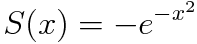 . This function is steep around x=[-2,2]. Updating alpha depends on the derivative of S, so steeper gradient will update faster. Large