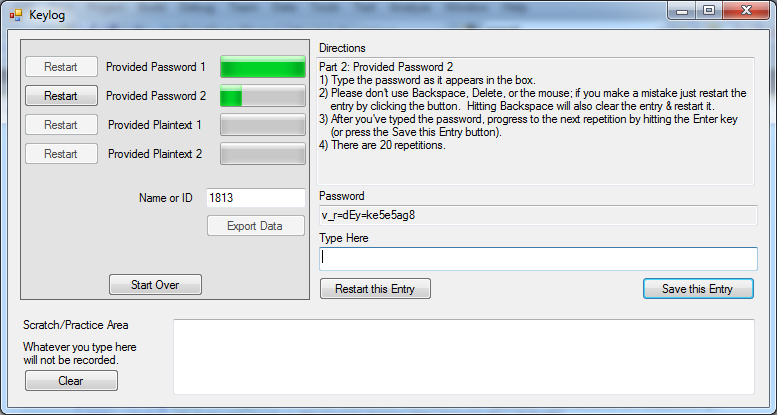
Figure 1: Data collection program, written in C#.
Keystroke Dynamics for User Authentication
COSC-174 Project Final Report, Spring 2012
Patrick Sweeney
Authenticating users on computer systems is an oft studied but still open issue. There's a generally accepted hierarchy of authentication mechanisms which range from the least secure to the most secure: [1, 2]
1) Authenticating via something you know.
2) Authenticating via something you have.
3) Authenticating via something you are.
This project attempts to determine the identity of a user based on how they type a password or passphrase. The characteristics of the user's typing (known as typing dynamics or keyboard dynamics) are examined and trained into machine learning algorithms to implement a form of biometric--something you are--authentication. By using hardware which is already present on computer systems (keyboard only) and measuring a process which users already do (typing), I hope to have a solution which is inexpensive, non-intrusive, and effective.
Machine learning algorithms are implemented for classifying users based on their typing dynamics, and the effectiveness of the models is compared based on passwords which are:
- Complex passwords of shorter length (8-12 characters) including letters, numbers, and special characters
- Complex passwords of moderate length (12-20 characters)
- Longer, text only, passphrases which exhibit more "steady state" or "natural" typing dynamics
- Longer passphrases which also contain some special characters
The overall objectives for the project are to:
1) Gather 10-20 typing data sets from volunteers, and
2) Use the collected data to train and test four implementations of multiclass support vector machines (SVMs), and
3) Examine the tradeoff of training time & classification time vs. success rate for the different password selections and different classification algorithms to draw conclusions about which technique(s) are best for various situations, and
4) Provide an interface to attempt "live" classification of a user with the trained algorithms.
My approach is presented in section 2, results in section 3, and section 4 draws final conclusions.
I wrote a dialog-based program in C# to collect typing metrics (see Figure 1). This program presents the user with four different passwords which will subsequently be referred to as Groups 1-4*:
- Group 1: Z83u#af3*b
- Group 2: v_r=dEy=ke5e5ag8
- Group 3: This sentence contains no special characters or numbers.
- Group 4: Everyone knows the answer to: 2+2=4
*Note: Group 5, referenced later, merges all data collected for Groups 1-4.
The program records the time that each key is pressed and released with millisecond accuracy. The user types in each password/passphrase 20 times, and then exports a data file with the raw keystroke data.
|
|
|
Figure 1: Data collection program, written in C#. |
A separate program is used to parse the raw data into set of 22 features. Some features were observed in other research [3, 4] and some are new/modified versions.
1) Mean key press duration for Keys other than Space and Shift
2) Mean key press duration for Space
3) Mean key press duration for Shift
4) Mean time between consecutive key-down events
5) Mean time between Shift-down and Key-down when Shift is used to modify a Key
6) Mean time between Key-up and Shift-up when Shift is used to modify a Key
7) Standard deviation of feature (1)
8) Standard deviation of feature (2)
9) Standard deviation of feature (3)
10) Standard deviation of feature (4)
11) Standard deviation of feature (5)
12) Standard deviation of feature (6)
13) Number of times Backspace is used
14) Total time to type the password/passphrase
15) Mean time between consecutive key-up events*
16) Standard deviation of feature (15)*
17) Mean overlap time (subsequent key is pressed before previous key is released)*
18) Standard deviation of feature (17)*
19) Mean time between alternating key-down events (i.e. time between a key-down event and the 2nd subsequent key-down event)*
20) Standard deviation of feature (19)*
21) Mean time between alternating key-up events*
22) Standard deviation of feature (21)*
*Added after midterm design review
Although metrics such as 1&4 are fairly standard in research, I introduce others such as 5&6 and make sure all the passwords provided an opportunity to exercise these sequences.
Four multiclass algorithms are implemented, all based on support vector machines (SVMs). I use Matlab's built-in SVM implementation for 1 vs. 1 comparisons, and extend it to perform the multiclass classification required.
1) One vs. Rest: In this implementation, the SVM is trained for one class at a time in a round-robin approach. All training examples are classified as either the class of interest, or not the class of interest, and the example is run through the trained SVM. Ideally only one class is identified as correct. However, it's possible that two or more similar classes are both identified as correct. It is also possible that NO classification is identified as correct.
Performance: scales linearly with N (where N is the number of classifications), however the large training sets increase the penalty of each comparison.
2) Max Wins: This algorithm pits each class against each other class in a 1 vs. 1 SVM. The "winner" of each comparison receives a vote, and the class with the most votes after all combinations have been tested is determined to be the winner [5]. Although this algorithm does guarantee at least one class will be selected as correct, it is also possible to have multiple "winners."
Performance: scales on the order of N2 as more classifications are added, though the training sets are smaller than in One vs. Rest.
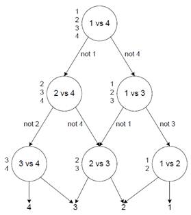
3) Directed Acyclic Graph (DAG): This approach is presented by Platt et al. in Large Margin DAGs for Multiclass Classification. DAG does multiclass classification via an efficient series of 1 vs. 1 comparisons based on directed acyclic graphs, as shown in Figure 2. A directed acyclic graph has directional edges and no cycles [6]. Each node represents a binary decision between the first class in the list of possible classes against the last class in the list. The losing class is eliminated, and the model proceeds to the next pairing.
Performance: scales linearly with N; for N classifications, (N-1) 1 vs. 1 classifications will be performed, and the smaller training set size can be maintained.
|
|
|
Figure 2: A DAG showing the process to find the best of four different classes [6]. |
4) Consensus Directed Acyclic Graph (CDAG): One shortcoming of the DAG algorithm is that the order of class comparisons can affect the outcome. In order to work around this, a consensus version of the DAG is implemented in which permutations of the class list are evaluated through DAG until a consensus of approximately N/3 is reached. After each random permutation of class comparison order is evaluated through DAG, the winner is given a vote similar to Max Wins. When any class receives floor(N/3) votes, that class is declared the winner.
Performance: an upper bound of (N-1)*(N-1) iterations of DAG is enforced, and a lower bound of floor(N/3) is possible. Each iteration of DAG requires (N-1) 1 vs. 1 classifications.
As noted, the One vs. Rest and Max Wins algorithms could possibly present 2 or more candidate classes as equally likely. In order to resolve these ambiguous results, sets of equally likely classes are passed to a DAG which efficiently narrows the result to a single most likely class for the example. Another way to differentiate between classes is to choose the class which receives the highest value after SVM classification. I did not see an obvious way to do this using Matlab's SVM capabilities, so I looked into using another popular SVM library for Matlab, LIBSVM. This library was producing worse results than Matlab's built-in SVM functionality, which is why I chose to stick with Matlab's SVM functions and use a DAG for conflict resolution.
For each Group, the 20 examples collected from each user are divided up into a training set and test set. Examples 1-5 are discarded as the user is just getting familiar with the phrase and probably hasn't built any rhythm. Examples 6-10 and 16-20 make up the training set, and examples 11-15 are used as the test set.
The training and test examples for every user are concatenated into one large training set and one large test set for each Group. In addition, a 5th Group of examples combines all test and training data from Groups 1-4 to examine generalized classification. The SVMs are trained on the data prior to any classification, and a classification is performed by passing the trained SVMs to an algorithm along with an example X to classify.
As described, each of the algorithms will provide a single most likely classification (or in rare cases, it is possible that no classification is found at all). The results are summed as either:
1) Correct: prediction given by the algorithm is the correct class for the example, or
2) Incorrect: either the wrong class was predicted or no match was made at all (only possible with One vs. Rest)
Along with the results listed above, the time is recorded to train the SVMs, and evaluate the training and test sets using each model.
I collected data sets from 11 volunteers. I had hoped to get closer to 20, but I did meet the minimum objective.
After encouraging initial results at the midterm, I made a few changes to improve the correct classification rates for the four models.
First I added features 15-22 to my training and test sets. However, I discovered through some trial and error that features 19-22 (mean time between alternating key down and alternating key up times) were not helpful. In fact, although they improved classification performance by approximately .5% on the training set, the performance on the test set was 1-2% worse depending on the Group. In addition, the added features caused a 5% penalty in SVM training time. Ultimately I dropped those four features.
Classification using features 1-18 was satisfactory, but I wanted to know if dropping any additional features would improve the classification performance. To answer this question, I performed 18 separate classifications of the test sets, leaving out one feature in each run. I discovered that by dropping feature 6 (mean time between key-up and shift-up sequences) I could improve the correct classification rate on the test set by approximately 2.2% on every algorithm except One vs. Rest, which was unaffected.
After narrowing my feature set down to 17, I tried another reduction but found that leaving out any other feature would make correct classification rates worse.
Finally, I wanted to optimize the SVM learning parameters boxconstraint and kktviolationlevel which can be optionally provided to Matlab's svmtrain function.
- boxconstraint (C): soft margin value for the SVM, default=1
- kktviolationlevel (kktv): fraction of examples allowed to violate the Karush-Kuhn-Tucker (KKT) conditions, default=0
I performed a classification on each Group's test set with the SVMs trained using values of C = {.125, .25, .5, 1} and kktv ={0, .01, .05, .1, .15, .2}. There was little variation in the results, as can be seen in Table 1. However, C=1 and kktv=.1 performed slightly better than other values, so that is what I implemented for my final training settings.
|
|||||||||||||||||||||||||||||||||||||||||||||
|
Table 1: Mean error rates across all 5 groups when SVMs are trained using parameters shown. |
|||||||||||||||||||||||||||||||||||||||||||||
The four models are evaluated based on the correct classification rate, the SVM training time, and the example classification time.
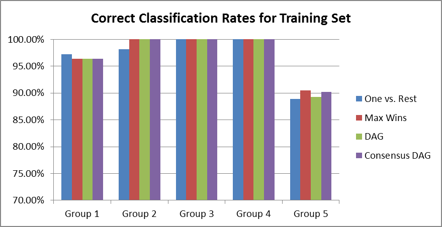
The One vs. Rest model did not perform as well as the other algorithms in most cases. See Figure 3 for a summary of the correct classification rates. Against the training set, this model outperformed all others by a small margin in Group 1 but otherwise underperformed. When classifying the test set, this model only performed well on Group 2, but whatever it gained for that Group it more than made up for in poor correct classification rates for Groups 1, 3, 4, and 5.
|
|
|
Figure 3: Correct classification rates for each model against Groups 1-5 in the training and test sets. |
The Max Wins model was usually either the best, or tied for the best, performer in each Group for both the training set and test sets. The only exceptions were the two scenarios where One vs. Rest outperformed all others (Group 1 training set and Group 2 test set) and Group 4 of the test set.
The DAG model was a mid-grade performer, tying the best results in Groups 2-4 of the training set and 3 & 5 of the test set. Dag also was never the worst performer in any scenario.
The Consensus DAG model was another mid-grade performer. Although it achieved the highest correct classification rate of any model against the test set (98% in Group 4), it was not consistently the highest (and in fact, was the worst performer against Group 2 in the test set).
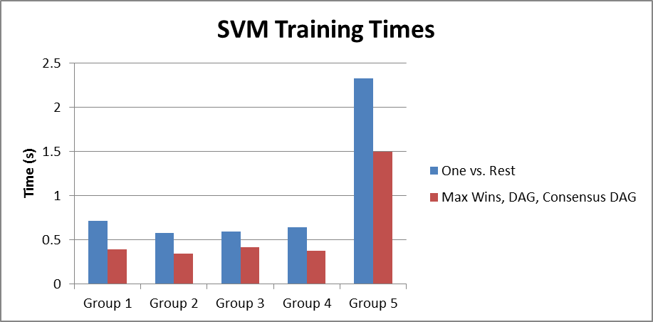
The training times for each model and each Group are shown in Figure 4. The Max Wins, DAG, and Consensus DAG all use the same set of 1 vs. 1 (class 1 vs. class 2, class 1 vs. class 3, etc.) trained SVMs, while the One vs. Rest uses the set of 1 vs. Rest SVMs (class 1 vs. not class 1, class 2 vs. not class 2, etc.). In addition, the One vs. Rest is penalized because it uses the set of 1 vs. 1 trained SVMs to perform disambiguation. As a result, it naturally shows a longer training time than the other models.
|
|
|
Figure 4: Model training times for 1 vs. Rest model and 1 vs. 1 based models which include Max Wins, DAG and Consensus DAG. In the 1 vs. 1 based models, .5*N(N-1)=55 SVMs of smaller size are trained. In the One vs. Rest model, N-1=10 larger SVMs are trained in addition to the 55 1 vs. 1 SVMs. |
As a side note, training times for the 1 vs. Rest SVMs were significantly affected by passing C and kktv options to Matlab'ssvmtrain function. When training SVMs for group 5, which has 440 samples, using options with svmtrain caused a 300% increase in SVM training time! The 1 vs. 1 training times were only affected by <10%. This explains why these training times seem inconsistent with those presented at the midterm, when I wasn't using options with svmtrain.
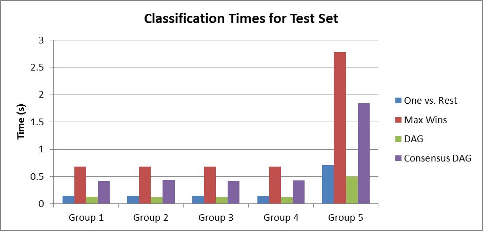
In this application, the training time can be frontloaded so a more important metric is classification time. Even the slowest models are quite fast for a single example classification; nevertheless, it would be ideal to have as short a classification time as possible. Figure 5 shows a comparison of classification times for the entire test set in each Group. Groups 1-4 in the test set have 55 examples, and Group 5 has 220 examples. The Max Wins model is the slowest, as expected, because it does the most comparisons (on the order of N2) for every example. Consensus DAG is not much better, while One vs. Rest and DAG perform the fewest SVM runs for each example. Overall DAG is the fastest model.
|
|
|
Figure 5: Runtimes which represent the amount of time for the Group's entire test set to be classified with the model (not including training time). Groups 1-4 have 55 test examples, while Group 5 has 220. Note that the training set has 2x as many entries as the test set, therefore the runtimes against the training set are approximately 2x what is shown for the test set. |
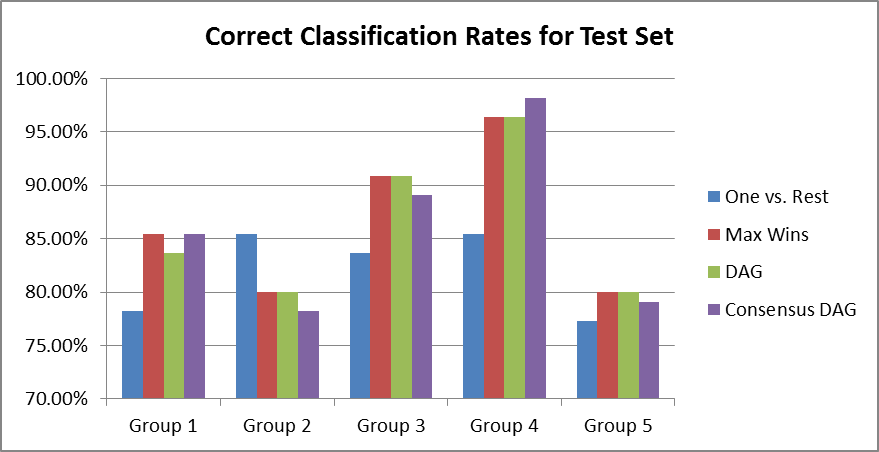
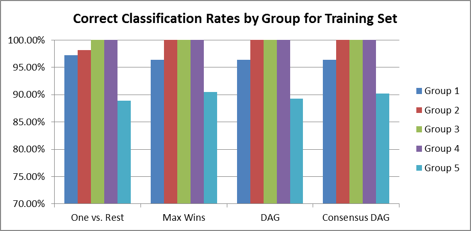
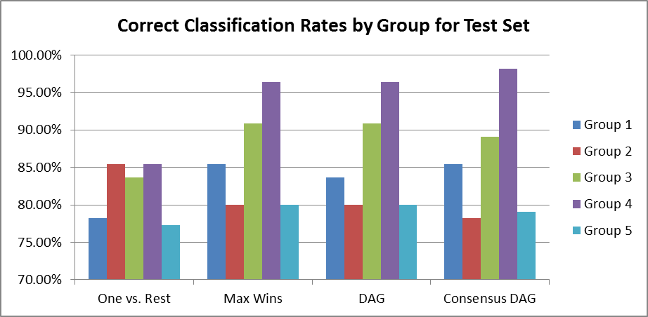
Figure 6 presents the same data as Figure 3, but arranged to compare the correct classification rates by password Group. Classification in the training set is perfect--100%--for all models in Groups 3&4 (longer passphrases). Additionally, all but the One vs. Rest model are able to correctly classify 100% of the Group 2 training examples. Group 5 classifications are a bit lower, which is expected because we're training the SVMs with examples from all of Groups 1-4 to attempt more generalized classification.
In the test set, correct classification rates are a bit lower across the board, but still reasonably good. The Group 4 passphrase (natural text with a few numbers and symbols) turned out to be the most easily identified style for all models (tied with Group 2 for the One vs. Rest model). Group 3 (natural text with no numbers or symbols) was second best for all but the One vs. Rest model. Surprisingly, the short alphanumeric/symbolic password (Group 1) was more easily classified in the test set than the longer password of the same style (Group 2).
|
|
|
Figure 6: Correct classification rates for each password Group, shown for each model. The Group 4 password (longer passphrase with some numbers and symbols) proved the easiest to classify. |
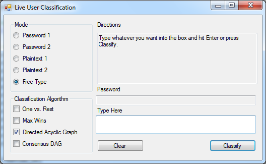
Although it wasn't originally a goal of the project, I decided to implement an interface which would attempt to classify users based on "live" input. Figure 7 shows the input dialog. Users can choose to enter one of the 4 passwords/passphrases that the models are trained on, or type free text of their choosing. When training the SVMs for the Live Check, I used typing examples 6-20 as the training set since I did not need to use some as a test set.
|
|
|
Figure 7: Live Check dialog, written in C#. |
I did not arrange any comprehensive testing of the Live Check system, but asked a few of the previous volunteers to try it. When using a previously learned password/passphrase, the correct classification rates were only around 50% at best. Just as in the test and training sets, I had the best success with the Group 4 (plaintext 2) passphrase. I also discovered that if I typed in the same password repeatedly, then the correct classification rates improved. This indicates that the models are very sensitive to typing rhythm variations. When users volunteered to provide training and test data, they typed the same password 20 times in succession, which I believe allowed them to build a rhythm where their entries were similar.
I also made many attempts to classify myself based on free text typing. In this mode, the program trains the SVMs with the Group 5 set, and uses them to classify any random text that the user enters. This was surprisingly effective, in that it worked some of the time. I didn't expect my very limited training set to generalize well to other typing situations, but it was able to correctly classify me 10-20% of the time. On top of that, it was fairly consistent in guessing one of 3 users who I must type similar to. Of course, 10% is as good as I would hope to get with random guessing, so I don't put much faith in this system. However, I believe with a better training set this type of generalized classification would be possible.
This was an interesting experience, and I've drawn some conclusions about classifying users via typing dynamics using multiclass SVMs.
1) The models are sensitive to rhythm. It's possible that with more training data, the sensitivity could be reduced. However, although I was seeking an unobtrusive means of performing biometric authentication, collecting the training data was clearly a burden and it's not ideal to ask users to type in even more repetitions to better train the system. The simple fact that I was unable to obtain good classification results with the Live Check a few weeks after the users originally submitted the training data demonstrates the lack of robustness in my system.
2) Longer passphrases that exhibit more natural typing dynamics provide better differentiation among users. I did expect this to be the case, however I was a little surprised that the sentence with numbers and symbols performed the best overall.
3) Any of the models would be suitable for this application based on training and classification times. Even though the training takes a couple of seconds (at most) that's only done once so it's frontloaded. If the models were modified to continuously update and learn, it might be more of an issue. Similarly, any of the models would be suitable based on classification times; they're all very fast for a single example.
Ultimately, I think the idea of using typing dynamics as a biometric has merit but my method of data collection is flawed. A different approach, wherein the user's typing is observed continuously and trained on a much larger data set (e.g. a week's worth of typing) may prove to be more useful. As designed, there's too much variation in the way users type based on factors which are hard to model when collecting data for the training set. For example, to account for how a user's typing characteristics change over the course of a day, I might have asked them to type a password once per hour while doing other tasks in between. Although this might provide a more robust training set, it would be arduous and probably not well received by the users.
All the same, I was impressed by the results of classifying the test set as it was, and think in that regard the project was a success. If I were pursuing this research in my career, I would be encouraged to continue. Certainly the end goal of cheap biometrics is a strong motivation.
|
[1] |
Shepherd, S.J.,
"Continuous authentication by analysis of keyboard typing
characteristics," Security and Detection, 1995., European Convention
on , vol., no., pp.111-114, 16-18 May 1995 |
|
[2] |
Crawford, H.,
"Keystroke dynamics: Characteristics and opportunities," Privacy
Security and Trust (PST), 2010 Eighth Annual International Conference on
, vol., no., pp.205-212, 17-19 Aug. 2010 |
|
[3] |
Ilonen, J., "Keystroke
dynamics," Advanced Topics in Information Processing-Lecture, 2003 |
|
[4] |
Bergadano, F., Gunetti, D., and Picardi, C.,
"User authentication through keystroke dynamics," ACM Trans. Inf. Syst. Secur.
5, 4 Nov. 2002 |
|
[5] |
Friedman, F.H.,
"Another approach to polychotomous classification",
Technical report, Stanford Department of
Statistics, 1996 |
|
[6] |
Platt, J., Cristanini, N.,
Shawe-Taylor, J., "Large margin DAGs for multiclass classification," Advances in Neural
Information Processing Systems 12. MIT Press pp. 543-557, 2000 |
|
|
Group 1 |
Group 2 |
Group 3 |
Group 4 |
Group 5 |
|
One vs. Rest |
97.27% |
98.18% |
100.00% |
100.00% |
88.86% |
|
Max Wins |
96.36% |
100.00% |
100.00% |
100.00% |
90.45% |
|
DAG |
96.36% |
100.00% |
100.00% |
100.00% |
89.32% |
|
Consensus DAG |
96.36% |
100.00% |
100.00% |
100.00% |
90.23% |
|
Group 1 |
Group 2 |
Group 3 |
Group 4 |
Group 5 |
|
|
One vs. Rest |
78.18% |
85.45% |
83.64% |
85.45% |
77.27% |
|
Max Wins |
85.45% |
80.00% |
90.91% |
96.36% |
80.00% |
|
DAG |
83.64% |
80.00% |
90.91% |
96.36% |
80.00% |
|
Consensus DAG |
85.45% |
78.18% |
89.09% |
98.18% |
79.09% |
|
|
Group 1 |
Group 2 |
Group 3 |
Group 4 |
Group 5 |
|
One vs. Rest |
0.72 |
0.58 |
0.59 |
0.64 |
2.33 |
|
Max Wins, DAG, Consensus DAG |
0.39 |
0.35 |
0.42 |
0.38 |
1.50 |
|
|
Group 1 |
Group 2 |
Group 3 |
Group 4 |
Group 5 |
|
One vs. Rest |
0.30 |
0.29 |
0.28 |
0.28 |
1.42 |
|
Max Wins |
1.36 |
1.35 |
1.35 |
1.35 |
5.55 |
|
DAG |
0.25 |
0.25 |
0.25 |
0.25 |
1.02 |
|
Consensus DAG |
0.83 |
0.83 |
0.83 |
0.83 |
3.47 |
|
|
Group 1 |
Group 2 |
Group 3 |
Group 4 |
Group 5 |
|
One vs. Rest |
0.15 |
0.15 |
0.14 |
0.14 |
0.71 |
|
Max Wins |
0.68 |
0.68 |
0.68 |
0.68 |
2.78 |
|
DAG |
0.12 |
0.12 |
0.12 |
0.12 |
0.51 |
|
Consensus DAG |
0.42 |
0.44 |
0.42 |
0.43 |
1.84 |