
Can Twitter Data Predict the Market?
Final Write-up
By Andrew Hannigan and Taylor Sipple
Problem Statement
Predicting the future price of securities is a foundational problem in quantitative finance. In recent years, new social media technologies have emerged as outlets for individuals to express their current mood, thoughts, and ideas. These new sources of data could contain valuable information about the general mood of the public and sentiment surrounding specific economic issues. Assuming that prices of government bonds are influenced by public mood and sentiment toward those countries, then perhaps we learn to predict global bond yield movements from sentiment or mood features on social media such as Twitter.
Bollen et. al. tested this theory by extracting general mood sentiments from Twitter posts and correlating those moods fluctuations to changes in the Dow Jones Industrial Average, achieving an 87.6% success rate in predicting the daily directional change of the DJIA [1]. Another study looked at correlations between sentiment towards specific companies and the price fluctuations in that company’s stock, and created a trading model that outperformed the DJIA [2]. We seek to implement and expand upon these methods to predict movements in both the DJIA and US Treasury bond yields.
Simplifying Assumptions
In designing our Tweet pre-processing algorithm, we made the following simplifying assumptions:
i. Mood states are independent.
Multi-dimensional views of mood have been widely advocated by psychologists as an instructive way to understand human mood [3]. A seminal study by Osgood et. al. showed that variance in mood and emotion can be simplified to three principal, independent dimensions: valence, arousal, and dominance [4]. To evaluate the mood content of a tweet, we will analyze the tweet with respect to these three mood dimensions.
ii. Tweets containing the phrases “feel”, “I am”, “be”, “being” and “am” are most likely to contain pertinent mood data. Tweets containing hyperlinks do not contain pertinent mood data.
These two assumptions were adopted from Bollen et. al. [1] because they appear to be a reasonable assumptions that have the purpose of cutting out noise from our very large data set. We believe that tweets containing hyperlinks are not emotionally pertinent because the focus of the tweet is the content contained within the hyperlink. The phrases noted above were chosen because we believe that they are an intuitive filtering mechanism for creating a subset of tweets that are highly likely to contain accurate mood data.
iii. Context is not required to analyze the emotional state of a tweet.
There has been recent research into analyzing tweet mood state by taking into account the context of words in a tweet. However, we are making this strong assumption because it has been used to great accuracy previously [1] and does require any additional expertise that we may be lacking.
iv. Words that are near-neutral for a given emotional state are not indicative of tweet mood.
We were concerned that the presence of a great number of near-neutral words (slightly positive or negative) could skew the data because they are not representative of the strong emotions people express. Additionally, we are less confident about the emotional scores assigned to these words. Therefore we excluded near-neutral words from our pre-processing algorithm. This methodology was also used by Danforth et. al, from whom we got this idea [5].
Data
For this project we have drawn data from several sources. For our Twitter data we are using the Stanford Network Analysis Project dataset, which contains over 476 million tweets collected from June through December 2009 [6]. We pulled data on the Dow Jones Industrial Average and US 10 Year Treasury Bond from Yahoo! Finance [7].
Tweet Pre-Processing
As previously stated, our dataset contains over 476 million tweets, which occupies 50 GB on disk. Due to memory constraints and the massive scale of this dataset, our pre-processing system is designed to process 1 GB chunks of tweet data at a time while updating a global python dict with unix days as keys and mood scores as values.[1]
In order to pre-process the tweets, we need to begin with a metric for judging the emotional content of words. The first metric we use is the Affective Norms for English Words (ANEW) corpus. This contains a valence, arousal, and dominance value for 1,030 common English words rated by subjects in a study by Bradley and Lang [3]. Valence is a rating on the happy-unhappy scale, arousal is a rating on the excited-calm scale, and dominance is a rating on the “in control”-controlled scale. The words selected for this study were chosen to include a wide range of words in the English language. The second metric is the labMT 1.0 corpus compiled by Chris Danforth at UVM. To construct this corpus, Danforth analyzed the New York Times from 1987 to 2007, Twitter from 2006-2009, Google Books, and song lyrics from 1960 to 2007, and extracted the 5,000 most commonly occurring words from each source. The union of these four sets of words resulted in a 10,022 word set that was the basis for his corpus. Danforth then used Amazon Mechanical Turk to obtain 50 valence ratings for each word in his set. The average of these ratings became the valence value for each term. Significantly, the valence values of ANEW and labMT are highly correlated, with a Spearman’s correlation coefficient of 0.944 and p-value < 10-10 [5]. For our purposes, we use the labMT corpus to compute valence because it contains ten times more words than ANEW. For arousal and dominance, we use the ANEW corpus.
In order to allow the ANEW corpus to apply to as many words as possible, we employ porter stemming on the ANEW key words and the tweet words. Using porter stemming, the words “happy” and “happiness” are both converted into the common stem “happi”. Using this method, we convert the ANEW word lookup table into a stem lookup table. This allows us to compute the ANEW mood values for many words, which increases the accuracy of our mood predictions for each day. We use the stemming-1.0 python library to implement these stemming methods [9]. Note that it is not necessary to stem the labMT corpus. Because the words for this corpus were selected based on frequency, the mood scores for the most common forms of each stem of already been computed, obviating any need for stemming [5].
For each day, we filter out all tweets that contain ‘http:’ or ‘www.’, or do not contain a personal word “feel”, “I’m”, “Im”, “am”, “be”, or “being”. The former rule is to avoid spam tweets, and the latter rule is to target a subset of tweets that is highly likely to contain content indicative of that user’s personal mood. This is a technique borrowed from Bollen et. al [10]. After filtering the tweets, we concatenate all tweets from each day into single strings and compute a mood score for each mood dimension using the following equation:
The following graph shows a scores for a given week from Tuesday to Monday of the following week:
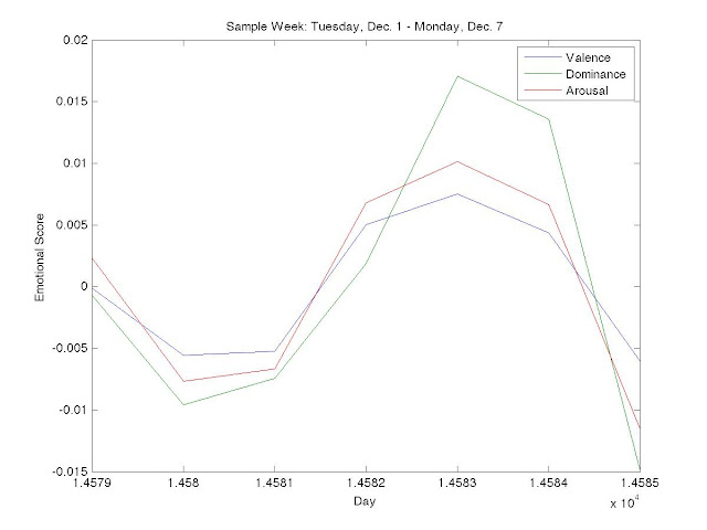
Fig. 1 - Example Week’s Mood Scores
While this is an imperfect science, we were encouraged by the cyclical results seen above. We see that values for valence, dominance and arousal dip midweek and spike on the weekends, which intuitively matches up with our own perception of the workweek. Further, we were particularly interested in the lagged increase in dominance as compared to valence and arousal as the weekend approaches. We see that on Friday, December 4, 2009 (day 14582 since January 1, 1970), valence and arousal values increase greater than dominance, but on the following day (14583) dominance peaks above both. With dominance being a measure of “control” over one’s life, it makes sense to us that people would be happier and more excited (valence and arousal) as the weekend approaches, but would not feel control (dominance) until the workweek is finished and they are absolutely free on Saturday.
Another way we spot-check the accuracy of our results is by comparing them to a study by Bollen et. al. in which they they checked how their computed mood timeseries correlated to major events such as the Presidential Election and Thanksgiving [10]. The following graph shows mood scores plotted for mood scores for all days between June 16th and December 31st. The weekly oscillatory mood scores are still apparent, but the mean score for each week varies. Additionally, seemingly random spikes in mood scores tend to correspond with holidays.
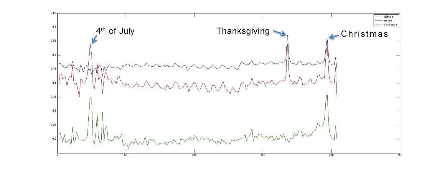
Fig. 2 - Full mood series with event labels
Learning Algorithm
We implemented our own Artificial Neural Network algorithm in Matlab as a classifier to predict whether a given security would move up or down on a given day. There are several steps in designing a Neural Network for usage, which are detailed below.
i. Algorithm Design
To implement the Neural Network we created two classes in Matlab - the neural network and the layer. The layer class contains the most granular information of the network, including the weights, number of nodes, learning rate, activation function and pointers to both the previous and next layers in the network; among other properties. It also includes basic methods to perform steps in feeding forward inputs through the network and for error backpropagation. The neural network class is designed to store the number of neurons in each layer as well as pointers to the input layer and output layer which allows us to traverse the doubly-linked layers in both the forward and backward directions. The network class contains methods to initialize a network with random weights, propagate inputs through the entire network, backpropagate error through the nodes and update weights based on the error backpropagation signal.
Further detail can be found in the code library submitted with this report under NeuralNet.m and Layer.m.
ii. Proof of Concept
Having coded up our Neural Network algorithm, we sought initial validation of our implementation by training a Neural Network on the Parkinson’s disease data from Homework 1. We achieved a 6% error over repeated trials, while the original study achieved an 8.2% error. Below the error over the training and test sets is plotted for the training of this network.
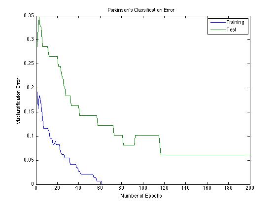
Fig. 3 - Parkinson’s Classification Error on 22-15-10-1 Neural Network
iii. Parameter Selection
It is important to begin this discussion by noting that parameter selection in a neural network is as much art as science. We sought to choose size of the network and learning rate in as scientific a way as possible, but admit that there is a limit to the scientific method in neural networks.
We first aimed to choose a learning rate that would be suitable for many sizes of neural networks that was sufficiently large to decrease convergence time while avoiding local minima. After much tinkering we found that 5x10⁻² satisfied these criteria - to validate this we tested a range of learning rates between 10-3 and 10-1 on 25 distinct two-layer neural network configurations and found that 5x10⁻² was the only step-size to achieve accuracies above 60%, reaching that level of accuracy 12.5% of the time.
Next we wanted to find a neural network configuration that would produce consistent results, avoiding overfitting and over-complexity such that the network would train within a reasonable timeframe. Selecting the configuration of a neural network is a bit of an art and a science. However, in order to make this decision as rigorously as possible, we tested nearly 500 network configuration with both 2 and 3 hidden layers and ascertained that an n-7-8-1 network was suitable for our purposes as it consistently achieved the lowest test error.
iv. Data Inputs and Outputs
The neural net takes the past six days of opening security price percent change along with the past six days of mood scores for whichever moods we are testing. We train the neural net on five different configurations of mood data: no mood, only valence, only arousal, only dominance, and all mood. Our neural net outputs a guess as to whether the security price will increase or decrease for a given day, with 1 corresponding to an increase, and a 0 corresponding to a decrease. Since our output is determined by a sigmoid function, we round our network output in order to generate a strictly binary prediction output.
v. Regularization
During our initial tests on the applying our n-7-8-1 neural net to stock and mood data, we found that we were suffering from severe overfitting problems. While our initial dataset was enormous, after processing the data into daily mood scores, we were left with only 205 days of twitter data, and only 146 were weekdays with corresponding DJIA and US Treasury data. Thus our final training dataset of size 121 was relatively small. This is what we attributed our overfitting problem to.
In order to solve this, we used “jittering” on our data, a technique that artificially boosts the size of a dataset by applying gaussian distributed noise to the X inputs while leaving the Y outputs unaffected [11,12]. For a given mxn X matrix, we made four independently generated mxn Z matrices with entries generated by a gaussian with covariance matrix 0.01 for all diagonal entries and a mean of 0. Each of the four Z matrices was added to X, introducing slight perturbations to our data. We combined these four new X matrices and trained our neural net with this new dataset. Using jittering, we were able to artificially quadruple the size of our training set, which improved our results and prevented overfitting. Below are figures showing our unjittered and jittered data training the neural network.
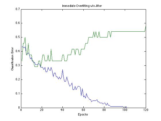
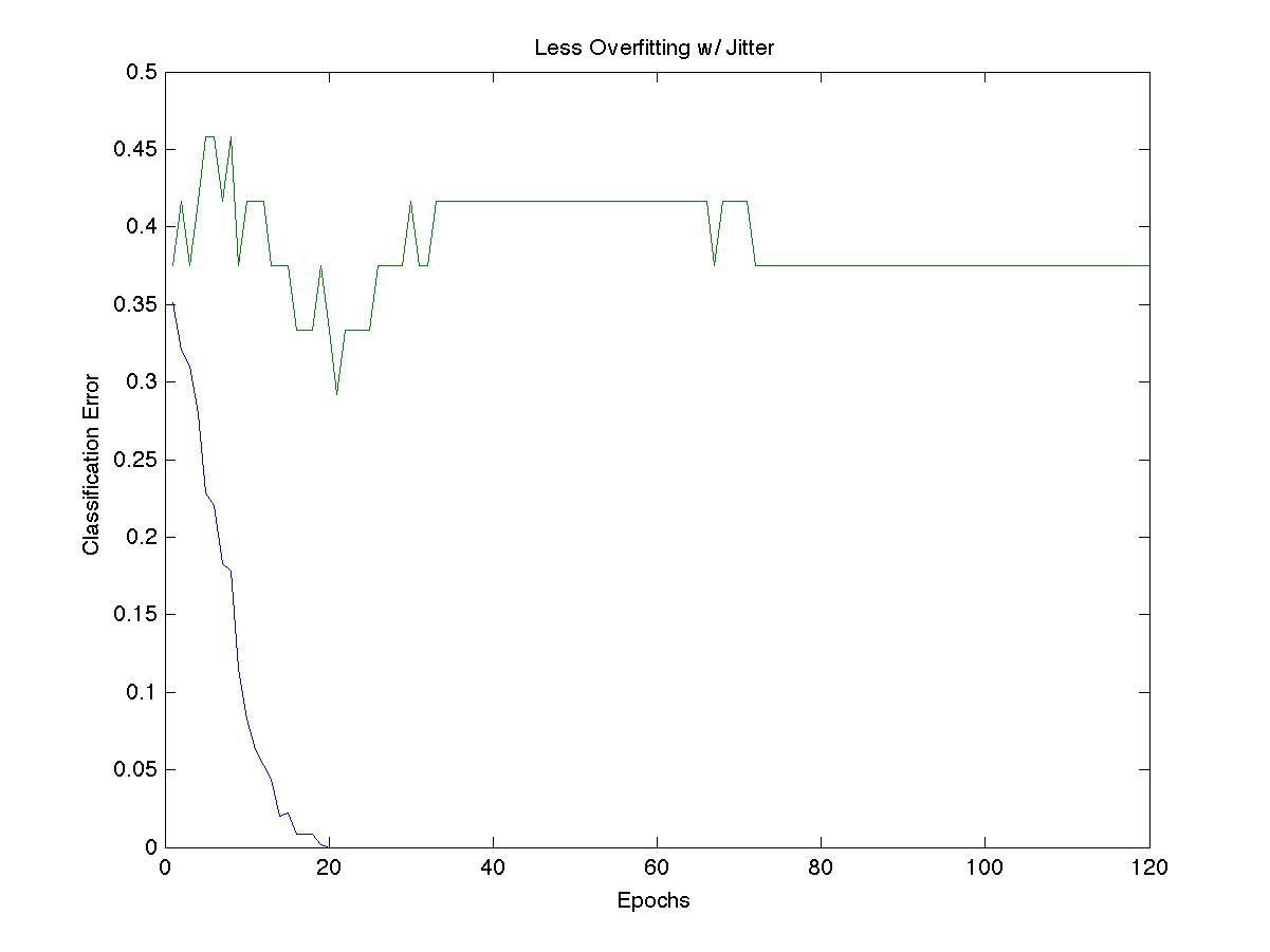
Fig. 4 - Overfitting reduction over 120 epochs by introducing jitter
With jittered data, we see less dramatic overfitting effects. While the jittered data still overfits during early epochs, the error only increases to 42% compared with 57% for the non-jittered data. Additionally, over the course of training, the jittered data is able to reach a stable error of 29% after about 1000 epochs of training. The unjittered data did not show this improvement in error after overfitting. Interestingly however, both jittered and unjittered data both achieve the same minimum test error of 29% before beginning to overfit. This suggests that an early stopping method may have also been an effective way to prevent overfitting.
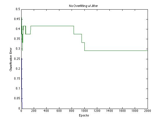
Fig. 5 - Overfitting reduction with jitter over 2000 epochs
Results
Training over 1500 epochs on the n-7-8-1 network with jittered data and the different input configurations specified above, we achieved the following maximum levels of accuracy in predicting directional movements in the Dow Jones Industrial Average and US Treasury bond market:
n-7-8-1 Network | DJIA Accuracy | US Treasury Accuracy |
No Mood | 54% | 50% |
Valence | 34% | 43% |
Arousal | 62% | 72% |
Dominance | 58% | 33% |
All Moods | 71% | 68% |
Table 1 - Predictive Accuracy of n-7-8-1 network over different input configurations
Our best results for predicting the Dow Jones were achieved by training the network with inputs from all mood dimensions, obtaining a 71% accuracy (P=0.0269)[2]. For US Treasury bonds, we achieved an accuracy of 72% (P=0.0138) using only the arousal mood dimension. Below we plot the training and test errors obtained throughout the training of the network over these different configurations.
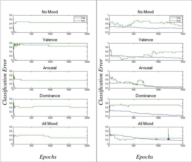
Fig. 6 - Classification Error vs. Epoch for Varying Mood Inputs
Conclusions
Our results suggest that Twitter mood data can in fact help predict fluctuations of prices in financial markets. Consistent with Bollen’s findings, we found that arousal was the best mood for predicting the directional change in the DJIA. To our knowledge, our study was the first that attempted to predict fluctuations in the bond market in addition to fluctuations in the stock market. Interestingly, we found that arousal is also most predictive for bond markets. This finding may suggest that arousal is a good predictor for financial markets in general, not just stock markets. However, since the bond and stock market are typically correlated, this finding may also just reflect the fact the bond and stock markets were particularly correlated during this period of time.
Next Steps
Steps for future exploration should involve increasing the sophistication of the Neural Network and implementing techniques to further improve the accuracy of the network at test time. One method suggested by Professor Torresani is to increase the size of the input vector by dividing the mood corpuses up to create separate but highly correlated input variables. In theory this would further stem the overfitting problem. Additionally, future studies could examine whether arousal is predictive for a market that not highly correlated with stock markets. This might show that arousal is a general indicator of financial market fluctuations.
Acknowledgements
We would like to thank Jure Leskovec for giving access to the SNAP database of Tweets. Most of all, we would like to thank Professor Torresani and our Teaching Assistant Weifu Wang for a fantastic class.
Citations
[1] Bollen, J., Mao, H. and Zeng, X.-J. 2010. Twitter mood predicts the stock market. Journal of Computational Science. http://arxiv.org/pdf/1010.3003v1.pdf
[2] Eduardo J. Ruiz et al., 2012. Correlating Financial Time Series with Micro-Blogging Activity. http://www.cs.ucr.edu/~vagelis/publications/wsdm2012-microblog-financial.pdf.
[3] Bradley, M. M., & Lang, P. J. (1999a). Affective norms for English words (ANEW): Instruction manual and affective ratings (Tech. Rep. No. C-1). Gainesville, FL: University of Florida, The Center for Research in Psychophysiology. http://bitbucket.org/mchaput/stemming
[4] Osgood, C., Suci, G., & Tannenbaum, P. (1957). The measurement of meaning. Urbana, IL: University of Illinois.
[5] Dodds PS, Harris KD, Kloumann IM, Bliss CA, Danforth CM (2011) Temporal Patterns of Happiness and Information in a Global Social Network: Hedonometrics and Twitter. PLoS ONE 6(12): e26752. doi:10.1371/journal.pone.0026752
[6] Leskovec, Jure. "Network datasets: 476 Million Twitter tweets." Stanford Network Analysis Project. Stanford University, n.d. Web. 12 Apr 2012. http://snap.stanford.edu/data/twitter7.html
[7] . "^TNX: Summary for CBOE Interest Rate 10-Year T-No." Yahoo! Finance. Yahoo!, 08 May 2012. Web. 01 May 2012. http://finance.yahoo.com/q?s=^TNX
[8] http://www.cmegroup.com/
[9] Matt Chaput. Stemming 1.0. http://bitbucket.org/mchaput/stemming
[10] Bollen, J., Pepe, A., & Mao, H. (2009). Modeling public mood and emotion: Twitter sentiment and socioeconomic phenomena. arXiv.org, arXiv:0911.1583v0911 [cs.CY] 0919 Nov 2009.
[11] Reed, Russel et al. (1992). Regularization Using Jittered Data. IEEE 1992.
[12] R.M Zur, Y Jiang, C.E Metz, Comparison of two methods of adding jitter to artificial neural network training, International Congress Series, Volume 1268, June 2004, Pages 886-889, ISSN 0531-5131, 10.1016/j.ics.2004.03.238.
[1] This process is well-suited for a parallel computing model such as a MapReduce where the map task produces a dict for a given chunk of data, and the reduce task combines all dicts into a single lookup table for mood scores on a given day. In order to process larger sized Twitter datasets, such parallel system would be invaluable.
[2] Using a binomial distribution with a p-value set to the proportion of days where the security price increased.