Recommendation Prediction in Social Networks
final write-up
Yangpai Liu & Yuting Cheng
Goal
We have two subproblems in our project. The goals are as following respectively:
- According to follow history of weibo, predicting whether or not a user will follow an item that has been recommended to the user .
- Predict the click-through rate (pCTR) of ads in Tencent search engine sousou.com
Data preprocessing
(Datasets are from [1]. Attributes of problem 1 are extracted and aggregated partly based on [2].)
Problem 1
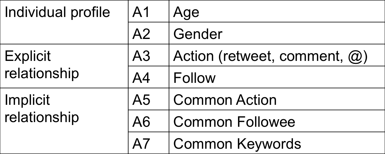
Figure 1. Attributes extracted from the data
Attribute 1: Year of Birth
$s(a_1) = 1-\frac{| yearofbirth(A) - yearofbirth(B) |}{100}$
Attribute 2: Gender
$s(a_2) = 1-| gender(A) - gender(B)|$
Attribute 3: Action
$s(a_3) = \begin{cases}1 & \text{if A takes an action to B or B takes an action to A} \\ 0 & \text{otherwise} \end{cases}$
Attribute 4: Follow
$s(a_4) = \begin{cases}1 & \text{ if A follows B or B follows A} \\ 0 & \text{otherwise} \end{cases}$
Attribute 5: Common Action
$s(a_5)=\frac{\textrm{number of common action objects}}{\textrm{total number of action taken by A and B}}$
Attribute 6: Common Followee
$s(a_6)=\frac{\textrm{number of common followees}}{\textrm{total number of followees of A and B}}$
Attribute 7: Common Keywords
$s(a_7)=\frac{\textrm{number of common keywords}}{\textrm{total number of keywords of A and B}}$
Problem 2
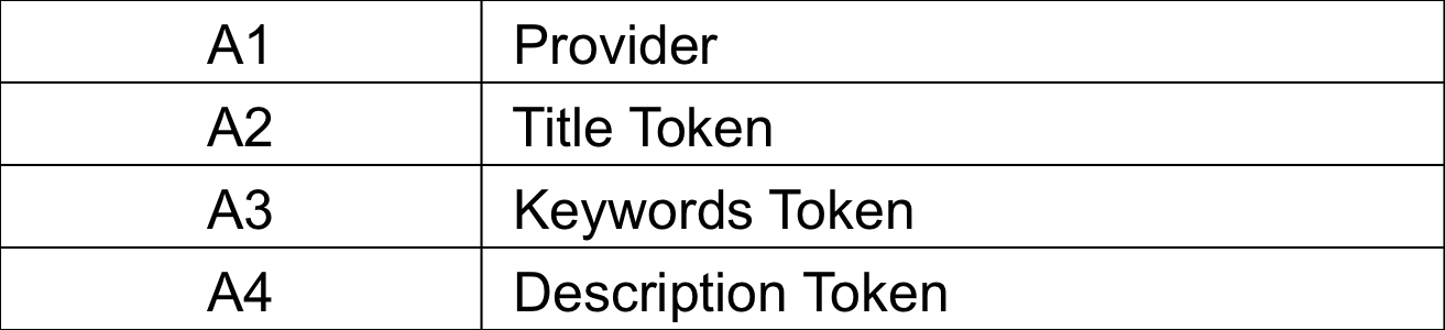
Figure 2. Attributes extracted from the data
Attribute 1: Provider
$s(a_1) = \textrm{# of common provider}$
Attribute 2: Title Token
$s(a_2) = \textrm{# of common title}$
Attribute 3: Keywords Token
$s(a_3) = \textrm{# of common Keywords}$
Attribute 4: Description Token
$s(a_4) = \textrm{# of common Description}$
Method: KNN + Metric learning
[need refine]
1. KNN classifier [3]
• if we want to decide if user A will "follow" item I, firstly, we find K nearest neighbor users in training set. Then, we will check if the number of users in the K neighbors who "follows" I is larger than a threshold. If so, the user A will "follow" I. Otherwise, A won't follow I.
Now we need to define the distance between user A and user B. We think the closer the two user are, the larger the similarity between them is.
Let s(A, B) denotes the similarity between A and B. To get s(A, B), we need to introduce several attributes we will use ($a_i$ denotes attribute i and s($a_i$) denotes similarity of attribute i between A and B):
• Select a subset of the users (neighbors) to use as predictors (recommenders).
We get the subset based on similarity. We define the similarity between user A and user B as follows:
$S(A, B)= \sum\limits_{i=1}^n w_i\cdot\textrm{similarity}(a_i, b_i)$
• Get the recommendation result.
If “majority” of the subset follow the item, then we predict the user will also “follow” the item. Otherwise, he/she will not follow the item.
About "majority": We tried to use some constant percentage as threshold to make the decision. It turns out quite bad when we have a bias of train set with some recommendations taken many times. Hence
We develop a way measure the "majority".
First we calculate the frequency of each item i in our trainset freq_i. For the item to handle in testset, we use following rules to get rid of the bias of high frequent items:
$$\textrm{result}=
\begin{cases}
1 & \textrm{ if } |\{i: \textrm{item} \in \textrm{Neighbor$(i)$.takeset}\}|> kc\cdot\textrm{item.freq} \\
0 & \textrm{ otherwise}
\end{cases}
$$
Note that c is a constant scaler used to get right prediction.
2. KNN regression [4]
Similarly, for a test ad, to predict its CTR, [3]
• Calculate the similarity between this ads and all ads in the training set.
• Calculate the top k most similar ads (i.e. neighbors).
• Predict the CTR from the average of the neighbor ads’ CTR:
$$\textrm{result}=\frac{1}{k}\sum_{i=1}^{k}\textrm{Neighbor$(i)$.ptr}$$
3. Distance metric learning [5]
We use metric learning to decide the weights of attribute in the KNN.
We want to learn $W=(w_1,\ldots,w_n).$ Define
$$ g(W):=g(w_1,\ldots,w_n)=\sum_{(x_i,x_j)\in S} || x_i-x_j ||^2_W-\log (\sum_{(x_i,x_j)\in D} ||x_i-x_j||_W),$$
where $||x-y||_W:=\sqrt{\sum_{i=1}^{n}(x_i-y_i)^2w_i}$, $S$ and $D$ are sets of similar and dissimilar pairs.
We minimize $g(W)$ subject to $W\geq 0$.
Results
1. Evalution methods
• We designed two benchmark for subproblem 1:
(1). Overall Correctness Rate (OCR):
$OCR=\frac{\textrm{number of correct prediction we make}}{\textrm{size of testing set}}$
(2). Recommendation Accept Rate (RAR):
$RAR=\frac{\textrm{number of correct "follow" prediction we make}}{\textrm{number of "follow" we make}}$
• We use Accumulative Error (AE) to evaluate methods for problem 2.
$AE=\sum_{i\in D}( \textrm{predicted click rate}_i- \textrm{actual click rate}_i)^2$
2. Experiment results
• Problem 1: Test for different attributes groups
In order to evaluate the attributes we extract, we launched a set of test with different attributes set. (i.e. with different w)
We can see that individual methods and the hybrid one (combine three kinds of attributes) have almost the same OCR (Figure 2). However, with hybrid method, we tend to have a higher RAR (Figure 3).
In other words, if we want build a positive recommendation system (make relatively regular number recommendation to users), the hybrid method has better performance.
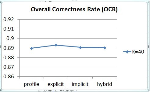
Figure 3. OCR of different attributes groups
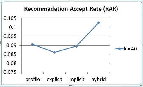
Figure 4. RAR of different attributes groups
• Problem 1: Uniform weighted distance vs. Metric learning distance w.r.t. K
When we test our hybrid methods on different K = {1, 5, 10, 20, 30, 40, 50}. The OCR of the test (Figure 4) and the RAR (Figure 5) has similar results. K = 1 and large K tend to have better performance on both benchmarks. K = 10,20,30 have a lower correctness rate.
The running time for different K is almost the same - we will obviously do the sorting when K is not trivially small.
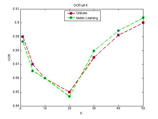
Figure 5. OCR of different K
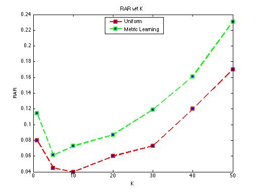
Figure 6. RAR of different K
We get at least 80% OCR for this problem. Combined with Distance metric learning, the RAR is improved significantly.
• Problem 2: Uniform weighted distance vs. Metric learning distance w.r.t K
We test uniform weighted distance vs. metric learning distance w.r.t K = {1, 10, 20, 30, 40, 50} on KNN-regression.
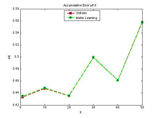
Figure 7. AE of different K
We get fair enough result for problem 2. However Metric learning doesn’t introduce obvious improvement with the result.
References
[1] KDD Cup 2012, http://www.kddcup2012.org/.
[2] U. H. Karkada, Friend recommender system for social networks.
[3] K-nearest neighbor algorithm http://en.wikipedia.org/wiki/K-nearest_neighbor_algorithm
[4] K-nearest neighbors – Regression http://chem-eng.utoronto.ca/~datamining/dmc/ k_nearest_neighbors_reg.htm
[5] E. P. Xing, A. Y. Ng, M. I. Jordan and S. Russell, Distance metric learning, with application to clustering with side-information