Can Twitter Data Predict the Market?

Milestone Write-up

By Andrew Hannigan and Taylor Sipple

Problem Statement

Predicting the future price of securities is a foundational problem in quantitative finance. In recent years, new social media technologies have emerged as outlets for individuals to express their current mood, thoughts, and ideas. These new sources of data could contain valuable information about the general mood of the public and sentiment surrounding specific economic issues. Assuming that prices of government bonds are influenced by public mood and sentiment toward those countries, then perhaps we learn to predict global bond yield movements from sentiment or mood features on social media such as Twitter.

Bollen et. al. tested this theory by extracting general mood sentiments from Twitter posts and correlating those moods fluctuations to changes in the Dow Jones Industrial Average, achieving an 87.6% success rate in predicting the daily directional change of the DJIA [1]. Another study looked at correlations between sentiment towards specific companies and the price fluctuations in that company’s stock, and created a trading model that outperformed the DJIA [2].  We seek to implement and expand upon these methods to predict global bond yield movements.

Simplifying Assumptions

In designing our Tweet pre-processing algorithm with made the following simplifying assumptions:

i. Mood states are independent.

        Multi-dimensional views of mood have been widely advocated by psychologists as an instructive way to understand human mood [3].  A seminal study by Osgood et. al. showed that variance in mood and emotion can be simplified to three principal, independent dimensions: valence, arousal, and dominance [4].  To evaluate the mood content of a tweet, we will analyze the tweet with respect to these three mood dimensions.

ii. Tweets containing the phrases “feel”, “I am”, “be”, “being” and “am” are most likely to contain pertinent mood data.  Tweets containing hyperlinks do not contain pertinent mood data.

These two assumptions were adopted from Bollen et. al. [1] because they appear to be a reasonable assumptions that have the purpose of cutting out noise from our very large data set.  We believe that tweets containing hyperlinks are not emotionally pertinent because the focus of the tweet is the content contained within the hyperlink.  The phrases noted above were chosen because we believe that they are an intuitive filtering mechanism for creating a subset of tweets that are highly likely to contain accurate mood data.

iii. Context is not required to analyze the emotional state of a tweet.

There has been recent research into analyzing tweet mood state by taking into account the context of words in a tweet.  However, we are making this strong assumption because it has been used to great accuracy previously [1] and does require any additional expertise that we may be lacking.

iv. Words that are near-neutral for a given emotional state are not indicative of tweet mood.

We were concerned that the presence of a great number of near-neutral words (slightly positive or negative) could skew the data because they are not representative of the strong emotions people express.  Additionally, we are less confident about the emotional scores assigned to these words.  Therefore we excluded near-neutral words from our pre-processing algorithm.  This methodology was also used by Danforth et. al, from whom we got this idea [5].

Data

        For this project we have drawn data from several sources.  For our Twitter data we are using the Stanford Network Analysis Project dataset, which contains over 476 million tweets collected from June through December 2009 [6].  For our bond data we have pulled data from Yahoo! Finance [7] and intend on retrieving further data from the CME Group [8] and the Bloomberg Terminal located in the Feldberg Business & Engineering Library.

Tweet Pre-Processing

As expected, tweet pre-processing has taken the majority of our time thus far.  As previously stated, our dataset contain over 476 million tweets, which occupies 50 GB on disk.  Due to memory constraints and the massive scale of this dataset, we have designed the pre-processing methods so that we minimize memory usage.  

In order to pre-process the tweets, we need to begin with a metric for judging the emotional content of words.  The first metric we use is the Affective Norms for English Words (ANEW) corpus.  This contains a valence, arousal, and dominance value for 1,030 common English words rated by subjects in a study by Bradley and Lang [3].  Valence is a rating on the happy-unhappy scale, arousal is a rating on the excited-calm scale, and dominance is a rating on the “in control”-controlled scale.  The words selected for this study were chosen to include a wide range of words in the English language.  The second metric is the labMT 1.0 corpus compiled by Chris Danforth at UVM.  To construct this corpus, Danforth analyzed the New York Times from 1987 to 2007, Twitter from 2006-2009, Google Books, and song lyrics from 1960 to 2007, and extracted the 5,000 most commonly occurring words from each source.  The union of these four sets of words resulted in a 10,022 word set that was the basis for his corpus.  Danforth then used Amazon Mechanical Turk to obtain 50 valence ratings for each word in his set.  The average of these ratings became the valence value for each term.  Significantly, the valence values of ANEW and labMT are highly correlated, with a Spearman’s correlation coefficient of 0.944 and p-value < 10^(-10) [5].  For our purposes, we use the labMT corpus to compute valence because it contains ten times more words than ANEW.  For arousal and dominance, we use the ANEW corpus.

        In order to allow the ANEW corpus to apply to as many words as possible, we employ porter stemming on the ANEW key words and the tweet words.  Using porter stemming, the words “happy” and “happiness” are both converted into the common stem “happi”.  Using this method, we convert the ANEW word lookup table into a stem lookup table.  This allows us to compute the ANEW mood values for many words, which increases the accuracy of our mood predictions for each day.  We use the stemming-1.0 python library to implement these stemming methods [9].  Note that it is not necessary to stem the labMT corpus.  Because the words for this corpus were selected based on frequency, the mood scores for the most common forms of each stem of already been computed, obviating any need for stemming [5].

For each day, we filter out all tweets that contain ‘http:’ or ‘www.’, or do not contain a personal word “feel”, “I’m”, “Im”, “am”, “be”, or “being”. The former rule is to avoid spam tweets, and the latter rule is to target a subset of tweets that is highly likely to contain content indicative of that user’s personal mood.  This is a technique borrowed from Bollen et. al [10].  After filtering the tweets, we concatenate all tweets from each day into single strings and compute a mood score for each mood dimension using the following equation:

Here, vi is the value for moodi for a given day where  wj is jth word in the daily tweet string.  Di is a lookup table with words as keys and moodi scores as output values.

        Due to the scale of our dataset, we have not yet finished pre-processing all of the data.  However, we ran our process on a small subset of Tweets from Tuesday, December 1 to Monday, December 7 to verify our method was working as expected.  For the three emotional states our process returned the following results:

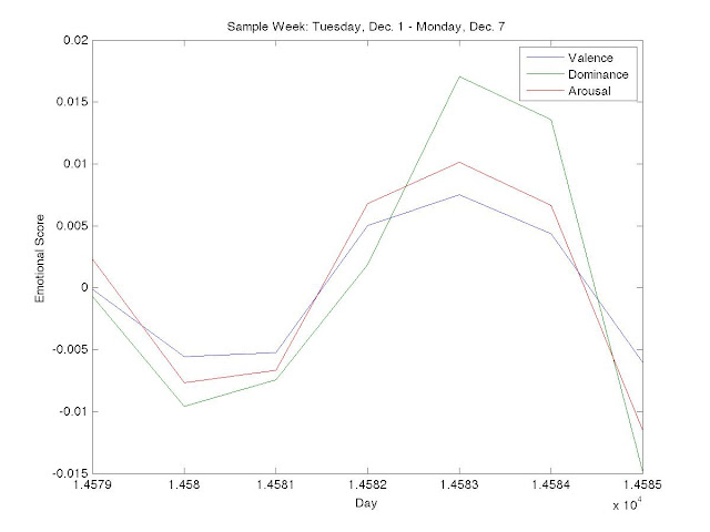
While this is an imperfect science, we were encouraged by the cyclical results seen above.  We see that values for valence, dominance and arousal dip midweek and spike on the weekends, which intuitively matches up with our own perception of the workweek.  Further, we were particularly interested in the lagged increase in dominance as compared to valence and arousal as the weekend approaches.  We see that on Friday, December 4, 2009 (day 14582 since January 1, 1970), valence and arousal values increase greater than dominance, but on the following day (14583) dominance peaks above both.  With dominance being a measure of “control” over one’s life, it makes sense to us that people would be happier and more excited (valence and arousal) as the weekend approaches, but would not feel control (dominance) until the workweek is finished and they are absolutely free on Saturday.  Another way we will spot-check the accuracy of our results is by comparing them to a study by Bollen et. al. in which they they checked how their computed mood timeseries correlated to major events such as the Presidential Election and Thanksgiving [10].

Learning

As of yet we have not chosen our non-linear learning algorithm.  Our original intention was to implement a Neural Network, but at the behest of Professor Torresani we are reconsidering due to the technical difficulties of implementing a Neural Network.

The first design choice we must make is whether or not to treat this learning problem as a classification or regression.  In the world of trading, it may be sufficient to predict the direction of market movement to a high degree of accuracy rather than its exact value.  By predicting the directional movement of a bond yield, we can convert our problem into a simple classification problem.  Bollen et. al. were able to predict the directional movement with 87.6% accuracy, suggesting that a classification approach is applicable to the problem of predicting changes in security prices.  

The second design choice is that of the model itself.  Our preliminary results from the pre-processing suggests a non-linear relationship between global bond yield movements and Twitter Mood because of the cyclicality seen in the latter that is not present in most financial time series as proposed in Arbitrage Pricing Theory [11].  We are still considering the Neural Network [12], but have expanded our sights to consider the use of a Support Vector Machine or more advanced Support Vector Regression [13].

Next Steps

Our immediate next step is to finishing running our pre-processing script and choose our non-linear learning algorithm.  The former will be completed within 24 hours from the submission of this paper.  The latter will be the subject of discussions over the rest of the week.  The design choice will be a combination of choosing whether to use a classification or predictive scheme.  Further discourse can be found in the section above entitled “Learning”.

By the final poster session we will have a robust learning algorithm and the results of training and testing the model on our bond data.  We will also seek to augment our pre-processing algorithm.  This may be accomplished by the inclusion of other emotional dimensions or changing the temporal characteristics of our processing.  While we cannot promise a strong predictive accuracy, we are encouraged by the results of Bollen et. al.  One way we will verify the accuracy of our model is by running our algorithm on data from the DJIA, which we hope will show levels of accuracy commensurate with that of Bollen et. al [1].

Sources

[1] Bollen, J., Mao, H. and Zeng, X.-J. 2010. Twitter mood predicts the stock market. Journal of Computational Science. http://arxiv.org/pdf/1010.3003v1.pdf

[2] Eduardo J. Ruiz et al., 2012. Correlating Financial Time Series with Micro-Blogging Activity. http://www.cs.ucr.edu/~vagelis/publications/wsdm2012-microblog-financial.pdf.

[3] Bradley, M. M., & Lang, P. J. (1999a). Affective norms for English words (ANEW): Instruction manual and affective ratings (Tech. Rep. No. C-1). Gainesville, FL: University of Florida, The Center for Research in Psychophysiology. http://bitbucket.org/mchaput/stemming

[4] Osgood, C., Suci, G., & Tannenbaum, P. (1957). The measurement of meaning. Urbana, IL: University of Illinois.

[5] Dodds PS, Harris KD, Kloumann IM, Bliss CA, Danforth CM (2011) Temporal Patterns of Happiness and Information in a Global Social Network: Hedonometrics and Twitter. PLoS ONE 6(12): e26752. doi:10.1371/journal.pone.0026752

[6] Leskovec, Jure. "Network datasets: 476 Million Twitter tweets." Stanford Network Analysis Project. Stanford University, n.d. Web. 12 Apr 2012. http://snap.stanford.edu/data/twitter7.html

[7] . "^TNX: Summary for CBOE Interest Rate 10-Year T-No." Yahoo! Finance. Yahoo!, 08 May 2012. Web. 01 May 2012. http://finance.yahoo.com/q?s=^TNX

[8] http://www.cmegroup.com/

[9] Matt Chaput. Stemming 1.0. http://bitbucket.org/mchaput/stemming

[10] Bollen, J., Pepe, A., & Mao, H. (2009). Modeling public mood and emotion: Twitter sentiment and socioeconomic phenomena. arXiv.org, arXiv:0911.1583v0911 [cs.CY] 0919 Nov 2009.

[11] Ross, Stephen (1976). "The arbitrage theory of capital asset pricing". Journal of Economic Theory 13 (3): 341–360. doi:10.1016/0022-0531(76)90046-6.

[12] Tung, W.L.; Quek, C.; , "GenSoFNN: a generic self-organizing fuzzy neural network," Neural Networks, IEEE Transactions on , vol.13, no.5, pp. 1075- 1086, Sep 2002 doi: 10.1109/TNN.2002.1031940. http://ieeexplore.ieee.org/stamp/stamp.jsp?tp=&arnumber=1031940&isnumber=22161.

[13] Smola, Alex, and Bernhard Scholkopf. "A tutorial on support vector regression." Statistics and Computing. 14. (2004): 199-222. Web. 8 May. 2012. http://eprints.pascal-network.org/archive/00000856/01/fulltext.pdf