On-Road Vehicle Detection in Static Images

Zhipeng Hu

Introduction

As vehicles improved with technological advancements, faster speeds were attained and more serious accidents were caused. Vehicle accident statistics disclose that the main threats a driver is facing are from other vehicles. Consequently, developing on-board driver assistance systems enabling vehicle collision avoidance and mitigation has attracted more attention. The most common approach to vehicle detection is using sensors such as radars and laser. However, they cost high to develop. Optical cameras, on the other hand, offer a more affordable and reliable solution. Visual information can be obtained without requiring any modifications to vehicles or road infrastructures. In this work, I will consider the problem of on-road vehicle detection from rear views of static images.

Methods

Gabor Wavelet Representation of Vehicles

I propose to use Gabor filters for feature extraction because it provides the best possible tradeoff between spatial and frequency resolution. Complex Gabor functions are complex exponentials with a Gaussian envelope. In this work, I take the Gabor wavelets defined as follows:

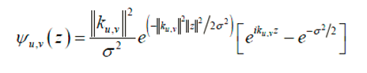
z = (x, y) and e is a function of oscillation, whose real part is the cosine function and imaginary part is a sine function. 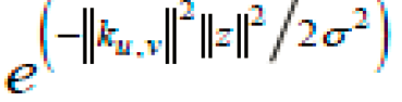is the Gauss function. The Gauss window reflects the localization of the Gabor filter both in the time and frequency domain, and limit the range of the oscillation function. Gabor filter can tolerate slight image distortion by using the Gauss window. 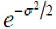is the DC composition which can be deduced to make the wavelet DC free. k_μ,v is the wave-vector of the filter corresponding to orientation μ and scale v . Through choosing a series of k_μ,v a set of Gabor filter can be obtained. σ is a constant that portray the wavelength of the Gauss window. Here I choose σ = 2π. k_{μ ,v} can be further written as

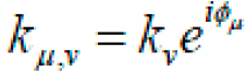
where k_v = k_max / f ^v and φμ = πμ / 8. k_max is the maximum frequency, and f is the spacing factor between kernels in the frequency domain. Different v is chosen to describe different wavelength of the Gauss window, and then control the scale of sampling. Different μ is chosen to describe the oscillation function with different direction, and then control the orientation of sampling. In this work, I use Gabor wavelets at five different scales, v ∈{0,...,4}, and eight different orientations, μ ∈ {0,...,7}. Five scales and eight orientations generate 40 filters. Figure 1. shows the real part of the 40 Gabor kernels with the following parameters: σ = 2π, k_max = π /2 and f = 2^1/2. The wavelets exhibit desirable characteristics of spatial frequency, spatial locality and orientation selectivity.

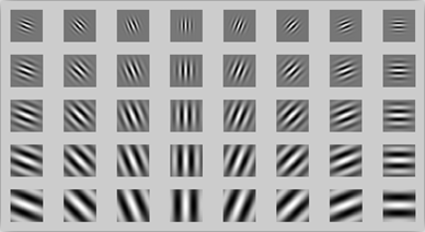
Figure 1. The real part of the Gabor kernels at five scales and eight orientations

The Gabor wavelet representation of an image is the convolution of the image with a family of Gabor wavelets. I convolve the image with complex Gabor filters in 5 spatial frequency and 8 orientation so that the whole frequency spectrum, both amplitude and phase can be captured. After convolution, local features can be represented by a set of convolution results at a certain convolution point which contains the important information at different orientation and scales. In Figure 2, an input vehicle image and the amplitude of the Gabor filter responses are shown.

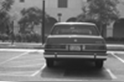
Figure 2(a). Original vehicle image

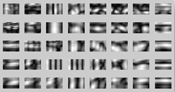
Figure 2(b). Filter response

Feature Extraction

I design support vector machine which prepares images for training phase. All data from both “vehicle” and “non-vehicle” folders will be gathered in a large cell array. Each column represents the features of an image while rows consist of file name, prepared feature vector for the training phase, and corresponding desired output of the network.

I adjust the histogram of the image for better contrast. Then the image will be convolved with Gabor wavelet by multiplying Gabor filters. However, despite the advantages of Gabor wavelet based algorithms in recognizing vehicle images with different illumination, scale and orientation, they require high computational efforts. The process of the convolution of a 21*32 pixel image with 40 Gabor wavelets remains a time consuming step and would become the main computation overloads for vehicle detection algorithm. Therefore, I use Fast Fourier Transform (FFT) and Inverse Fast Fourier Transform (IFFT) to speed up the computationally intensive convolution process, i.e., both Gabor wavelets and the image are transformed to frequency domain using FFT and the product is then transformed back to spatial domain using IFFT.

To save time, the family of Gabor wavelets has been saved in frequency domain before the convolution of the image. After performing convolution, the 40 Gabor filtered images are concatenated together to form a big 105*256 matrix of complex numbers which means that the dimension of the extracted Gabor feature would be incredibly huge, i.e., 26,880 for images with size 21*32 when 40 wavelets are applied. Consequently, dimensional reduction technique is used to reduce the dimension to a certain magnitude.

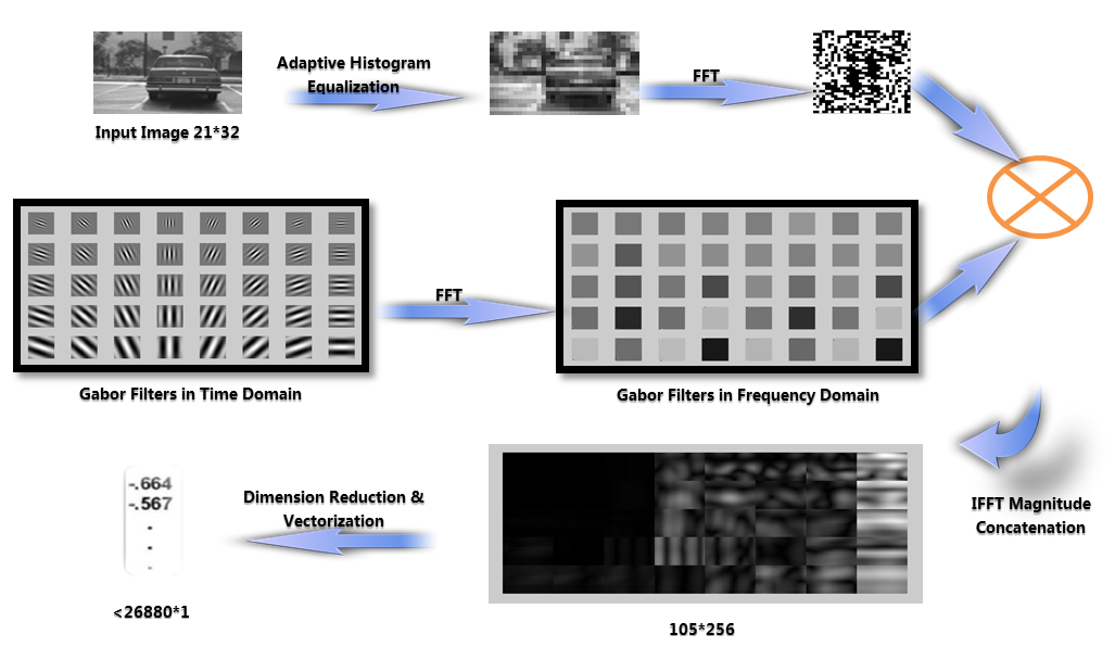
Figure 3. Steps involved in feature extraction

Classifier training

Once the dimension of an extracted feature vector has been reduced and discrimination ability enhanced by a certain subspace analysis, Support Vector Machine classifier could be applied for classification. SVMs are primarily two-class classifiers that have been shown to be an attractive and more systematic approach to learning linear or non-linear decision boundaries. Given a set of points, which belong to either of two classes, SVM finds the hyperplane leaving the largest possible fraction of points of the same class on the same side, while maximizing the distance of either class from the hyperplane. Assuming l examples from two classes:

Finding the optimal hyper-plane implies solving a constrained optimization problem using quadratic programming. The optimization criterion is the width of the margin between the classes. The discriminate hyperplane is defined as:

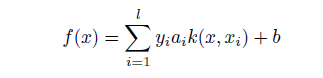
where k(x, x_i) is a kernel function and the sign of f(x) indicates the membership of x. Constructing the optimal hyperplane is equivalent to finding all the nonzero a_i. Any data point x_i corresponding to a nonzero a_i is a support vector of the optimal hyperplane. In this work, I use built-in function in bioinformatics tool box in Matlab to perform SVMs classifier training.

Milestone Summary

Achievement

• Dataset Collection and Preprocessing
• Gabor Wavelet Representation
• Gabor Feature Extraction
• SVM Training

What’s next?

• Feature Point Localization
• SVM Classification
• Image Scanning and Vehicle Detection

Remaining Timeline

• May 09 – May 20: Classification method implementation
• May 21 – May 30: Optimization, testing and final write-up

References

1. N. Matthews, P. An, D. Charnley and C. Harris, “Vehicle detection and recognition in greyscale imagery”, Control Engineering Practice, vol. 4, pp. 473–479, 1996
2. Z. Sun, G. Bebis and R. Miller, “On-road vehicle detection using Gabor filters and support vector machines”, IEEE 14th Int. Conf. Digital Signal Processing, Greece, pp. 1019–1022, 2002
3. Z. Sun, G. Bebis and R. Miller, “On-road vehicle detection using evolutionary Gabor filter optimization”, IEEE Transactions on Intelligent Transportation Systems, vol. 6(2), pp. 125-137, 2005
4. Yang Zhang, “Time Frequency Analysis Tutorial: Gabor Feature and its Application”
5. Linlin Shen, Li Bai, “A review on Gabor wavelets for face recognition”, Pattern Analysis and Applications, vol. 9(2), pp. 273-292, 2006
6. MIT CBCL Car Database, http://cbcl.mit.edu/software-datasets/CarData.html