Discriminative Random Fields for Aerial Structure Detection
Daniel Denton and Jesse Selover
The description and motivation of our project remain unchanged since the original proposal. Therefore, we will begin at the point where the proposal writeup ended, with the tasks we set for ourselves to complete by the milestone date.
Recap: Milestone Goal
When we began this project, we set out to complete the following tasks by the milestone date:
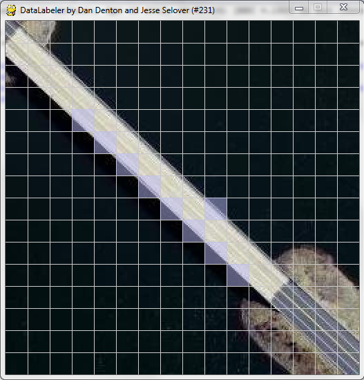
- Writing a short program to facilitate hand-labeling our data
- Hand-labeling the data
- Extracting features for each image (pre-processing)
- Coding the DRF model
- Training the DRF model
- Producing preliminary results
Now that the milestone date has arrived, we have completed almost all of these tasks. In short, we have written our data labeling program, and used it to label some (but not all) of our data. We have successfully extracted from our images the feature set that our DRF model uses to make its classifications. We have coded the complete algorithm, with both training and inference. We have trained the algorithm on the subset of data which we have labeled so far, although we this using a default selection of hyper-parameters which we eventually intend to discover using cross validation. Finally, we have used the trained model to classify sites on a few test images, and discovered that there is currently a bug in how we are applying the inference when we include the interaction potential term.
As long as we can find and fix our bug with the use of the interaction potential in a reasonable amount of time, we should be on track to tune the algorithm, and test its behavior on several datasets, including some used by previous researchers [1], [6].
Data Labeling
We began by deciding to use images of 256x256 pixels split into 256 16x16 pixel sites (the same site size used by Kumar and Hebert [6]). Since the images we acquired from the Montgomery County GIS website [8] were larger than this, we used a script to randomly crop each image to the desired size. We also had the same script randomly rotate each of our images, because we are interested in performing structure detection which is not dependent on compass orientation.
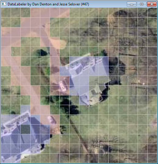
Since we need to label 16x16=256 sites for each image, and we intend to label 300 of our own images along with some images from the datasets of previous researchers, it was imperative that we create a tool which simplifies and speeds up the process of creating and storing site labelings. We decided to use python for our data labeling program, because the pygame library provides such great tools for easily creating a simple point and click application.
One idea that we have been playing around with is to try training the model with labelings of only buildings, and also with labelings which label every man-made structure (including roads, and driveways, etc.) to compare the results. Thus, we wrote the data labeler to allow us to use 3 labels, which form a totally ordered set:
- any_site
- any_structure
- building
By performing our labelings with these three labels, and choosing the most specific applicable label for each site, we can easily choose the threshold for either of the two binary classifications we are interested in training on.
The data labeler continuously backs up the current labeling of each image as a comma separated text file which we then read in our C# implementation. This allows the data labeler to load the latest labeling of any image. By outputting our inferred classifications of test images to this format, we gain the added benefit of using the same data labeler to display our classification results.
We now have the data labeler giving us all of the functionality that we foresee wanting from it. We have used it to label 80 of our training images that we could use to begin testing our algorithm. At this point, it simply remains to finish the labeling of the remaining images in our dataset.
The Kumar-Hebert dataset [6] has kindly been made available to us, and it comes pre-labeled. We hope to also get access to the dataset used by Bellman and Shortis [1]. Their images also are 256x256, but are only labeled with a single boolean variable for the presence of absence of a building. Thus, in order run our algorithm on their data, we will need to perform individual site labelings, which we can perform with our same data labeling program.
Image Features
We have implemented the single-site image features from [6] because they are most useful for comparison with other methods; we should be able to implement the multi-scale features with little additional trouble later.
The image features are all derived from an initial pixel-by-pixel gradient computation. To calculate the gradient vector at a pixel, we first convert the image to grayscale using NTSC-recommended values (Intensity = 0.299*R + 0.587*G + 0.114*B). Then to get the directional x-derivative, we convolve the resultant matrix of intensities with the derivative of a gaussian horizontally and the original gaussian vertically; the process is analogous for the directional y-derivative. We wrote code in C# to do this; we found no library to do it for us.
The variance of the gaussian is a hyper-parameter; we will have to optimize it. For now, we contacted Kumar and Hebert and they say they used 0.5 which seems like a decent, upstanding number that we don't really object to much. The algorithm is coded referencing the number only as a constant, so we can change it easily.
We bin the gradients of the pixels in each site into a histogram array indexed by orientations; we weight their contributions by their L2 norms. We chose to smooth the histogram with a simple triangular kernel, rather than the gaussian kernel of [6]; this will be very simple to change later.
The number of bins in the histogram is also a hyper-parameter; we can change it in the code by editing one variable. We chose 8 bins as a preliminary step, based on our research from [10]
Then the features we compute are heaved central-shift moments vp of the 0th through 2nd order. v0 is defined as the arithmetic mean of the magnitudes. Let the bins be Ei and let H(x) be the indicator function for the positive real numbers; then vp for p > 0 is defined as

In addition, we compute the absolute value of the sine of the angle difference between the two highest peaks of the histogram, to measure the presence of near-right-angle junctions.
In the original [6] paper, Kumar and Hebert also used the angle of the highest peak to perhaps allow their algorithm to catch on to the predominance of vertical lines in man-made structures in their data-set. However, our photos are not taken from upright cameras, houses did not tend to be aligned with the cameras, and in fact we randomly rotated the images in preprocessing to enforce this invariance, so we removed this feature. It should not be useful for our application; it would function as random noise.
As we said earlier, we only coded the single-site feature vector, but the remaining features from [6] were all simple functions of the pixel-wise gradient histograms, so we will be able to implement them if necessary.
Modified Model
We decided to use the modified DRF model presented in [6], as the learning objective is convex and it promised to be slightly easier to train. Kumar and Hebert suggest gradient ascent to maximize the log-likelihood, but we had to re-derive the gradients with respect to the vector parameters of the model.
In exchange, however, the algorithm for inference became slightly more technical. We were planning on using iterated conditional modes; iterating over the image assigning to each site the label of maximum likelihood given its neighbors. With the modified DRF model, though, you can compute exact MAP estimates of the labeling with an algorithm presented in [3] as mentioned in [6].
Training
We had a lot of fun re-deriving the gradient of the log likelihood to ascend it: We want to find

So we calculate:
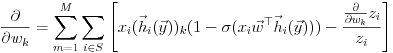
where

Similarly, for v,
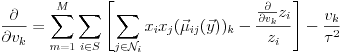
where

Issues with the Training
We had trouble for a while getting the training to converge; this turned out to be a bug not in our code but in our math. An incorrect application of the chain rule made w's gradient slightly off; when we fixed this, the gradient ascent worked very well. With our chosen convergence constants, it tends to converge in under five minutes. It takes a bit longer per iteration then we'd like, and we've only been training it on 80 images; its runtime should be proportional to the number of images, and we plan to use 200 for the final results. We used C# to serialize the w and v we find at each iteration to XML, so we can view the coefficients and save our progress when we run it for extended periods of time.
Inference
The [DRFS 2006] authors mentioned that the MAP estimate of the labeling could be computed exactly with an algorithm of Grieg et. al. However, that paper presented an algorithm for a different random field model, without the specific potential form of DRFs.
The algorithm works by creating a graph with image sites as nodes, plus a source node and a target node, and specifying edge capacities between the nodes in such a way that the equation for the capacity of a cut on the graph separating the source and the target is only an additive constant away from the equation for the negative likelihood of a labeling. There is a known algorithm to find the minimum cut, and when we have found it we have found the maximum likelihood labeling.
Specifically, according to the algorithm, lambda[i] is defined as the log-likelihood ratio at site i of the site being classified as structure; if lambda[i] is positive we create an edge from the source to the node i with capacity lambda[i], and if it's negative we create an edge from the node i to the target with capacity -lambda[i].
Then we create undirected edges between site nodes i and their neighbors j, with capacity beta[i,j] which is the coefficient of the interaction potential. Unfortunately, our interaction potential is not of that form.
In fact, the log likelihood ratio is of a different form as well. We rederived these edge weights in the context of the modified DRF model:
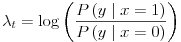
Using Bayes' rule we have

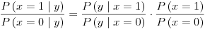
So
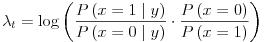
We started by assuming that the prior odds are fifty-fifty, so we got
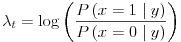

We are modeling P(x=1 | y) by Sigma(wT h(y)), so we derive that

Recently, however, we've investigated using empirically measured prior odds; it's had a noticeable impact on our classifications.
As for beta[i,j], we've used the analogue of the Ising-model coefficients for our specific interaction potential: max(0,vT * mu[i,j]y)
We implemented the min-cut algorithm for MAP label selection using C#. The algorithm is the standard Ford-Fulkerson min-cut using depth first search. After fixing a problem with the depth first search, the min-cut algorithm seems to be working swimmingly.
Unfortunately, the same cannot be said for the actual inference. We began solving the problem by setting all of the beta[i,j]s to zero, which performs inference using only the association potential and is analogous to logistic regression. When we did this, we got believable classifications:
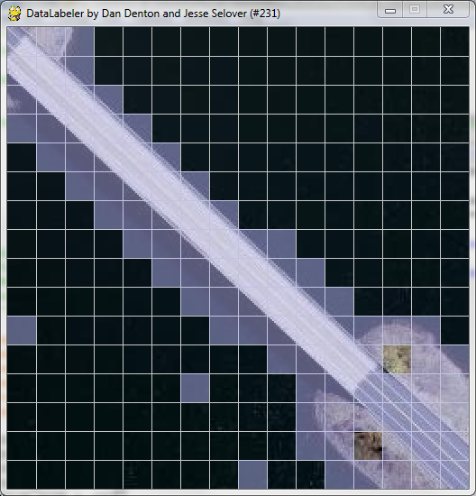
When we add in the beta[i,j]s calculated from the interaction potential, however, we are seeing behavior where the classifier will mark every site as being the same, either as all ones or all zeros. This means that, after the introduction of the beta[i,j]s, the min-cut is always either just the source vertex, or everything but the sink vertex. Clearly the beta[i,j]s are too large relative to the lambda[i]s. What we need to do is go over our derivations of these values to check whether we have computed these values correctly.
Our most recent theory for what is causing this mismatch is that we have not yet correctly set the hyper-parameter tau. Tau is the variance of the prior on the vector of interaction parameters, v. By using a smaller value of tau, we should cause v to take on smaller values relative to w, and hence cause the beta[i,j]s to shrink relative to the lambda[i]s. It remains to see whether this fixes the problem. Once we find the error, we expect that the DRF classifications using the interaction potential correctly will significantly outperform the logistic classifier.
Remaining Work
The highest priority right now is to discover the bug that exists in our use of the interaction potential for classification. Once we have that fixed, we will finally have access to the real results of the DRF classifier.
We took the time to individually download 300 orthophotos for our dataset. Of these, we have been using the 80 which we have already labeled for all of our training so far. We need to use the data labeler to label the remaining photos, and then train the model on our full training set (200 randomly selected images). Using cross validation with our training data, we will tune the variance of the gaussian gradient used for feature extraction, along with the variance of the gaussian prior on v, tau. With a tuned model, we hope to achieve classification rates similar to those obtained by [6]. We expect that it will be hard to actually achieve the combined 70.5% detection rate and 0.4% false positive rates that Kumar and Hebert got, because of the ambiguity of surfaces like roads and parking lots which sometimes have angular edges and sometime rounded edges. We hope, however, that when detecting just buildings we can get high detection rates, and when detecting all structures we can avoid most false positives.
After we finish with quantitative analysis of classification using our personal dataset, we will be ready to move on to other datasets for comparison. We have Kumar and Hebert's already labeled dataset, and we look forward to seeing what kind of results we can achieve on that data. We also need to contact Bellman and Shortis (we should probably do this very soon) to try to get access to their data. With proper labeling, we hope to compare our building recognition rates, where we will consider a success whenever the algorithm labels at least one site of an image containing a rooftop, or when it leaves blank every site of an image containing no rooftop.
Finally, we need to polish up and increase the commenting in our code, and prepare the final presentation. We believe that we are on track to accomplish all of this by the 30th.
References
- C. Bellman and M. Shortis. A machine learning approach to build- ing recognition in aerial photographs. In International Archives of the Photogrammetry, Remote Sensing and Spatial Information Sciences, pages 50-54, 2002.
- R. Cipolla, S. Battiato, and G.M. Farinella. Computer Vision: Detection, Recognition and Reconstruction. Studies in Computational Intelligence. Springer, 2010.
- C. Fox and G. Nicholls. Exact map states and expectations from perfect sampling: Greig, porteous and seheult revisited. In Proceedings MaxEnt 2000 Twentieth International Workshop on Bayesian Inference and Maximum Entropy Methods in Science and Engineering CNRS, May 2000.
- D. Greig, B. Porteous, and A. Seheult. Exact maximum a posteriori estimation for binary images. Journal of the Royal Statistical Society, 51:271-279, 1989.
- S. Kumar and M. Hebert. Discriminative random fields: a discriminative framework for contextual interaction in classification. In Computer Vision, 2003. Proceedings. Ninth IEEE International Conference on, pages 1150 -1157 vol.2, Oct. 2003.
- S. Kumar and M. Hebert. Discriminative random fields. International Journal of Computer Vision, 68(2):179-202, 2006.
- J. Lafferty, A. McCallum, and F. Pereira. Conditional random fields: Probabilistic models for segmenting and labeling sequence data. In C. Brodley and A. Danyluk, editors, ICML, pages 282-289. Morgan Kaufmann, 2001.
- Maryland GIS Montgomery County, April 2012.
- F. Shi, Y. Xi, X. Li, and Y. Duan. Rooftop detection and 3d building modeling from aerial images. In Advances in Visual Computing, volume 5876 of Lecture Notes in Computer Science, pages 817-826. Springer Berlin / Heidelberg, 2009.
- R. Szeliski. Computer Vision: Algorithms and Applications. Texts in Computer Science. Springer, 2010.