Milestone: Predicting Tennis Match Outcomes Through Classification
Shuyang Fang '14 sfang@cs.dartmouth.edu
Computer
Science 074/174: Machine Learning and Statistical Data Analysis - 2012S
Recap
Men's
tennis ATP rankings give some insight as to the quality of a given player.
However, rankings are not a definite guide to predicting match outcome.
Specifically, factors such as first serve percentage, tiebreak percentage, and
even incoming match record all offer additional insight to predicting the
winner of a match. The goal of this project is to instruct the computer to
predict the winner of a tennis match with greater accuracy than both random
guessing and ranking comparison.
Progress
I
am approximately on track with the goals I had set out for myself to accomplish
by this point. I have compiled the necessary match data as well as implemented
a strictly ranking prediction scheme as well as an Adaboost
generated model (although it is flawed).
Data
I
ended up deviating from the datasets I had intended to use due to a lack of
information. I am now using the match results from
http://www.tennis-data.co.uk/alldata.php
which contains all matches and results for ATP
seasons 2000-2012 (up to this point). For player info, I am using
http://statracket.net/?view=stats/stats.php
which provided a conveniently pre-compiled
dataset of ATP Matchfacts of the top 200 or so
players from 2004 to 2010. Using these two datasets in conjuction,
I created a 15-feature vector for any given match that includes the features I
deemed relevant/that were also attainable/documented. To clarify this, take
this match, the 2009 Australian Open final between Rafael Nadal
and Roger Federer.
|
Feature |
Value |
|
Winning% |
0.067 |
|
Tiebreak Winning% |
0.019 |
|
Matches Played |
10 |
|
Aces/Match |
-5.6 |
|
Double Faults/Match |
0.3 |
|
1st Serve% |
5 |
|
1st Serve Points Won% |
-5 |
|
2nd Serve% |
3 |
|
2nd Serve Pts
Won% |
2 |
|
ServeGames Won% |
-1 |
|
Break Points Saved% |
-1 |
|
Return 1st Serve Points Won% |
2 |
|
Return 2nd Serve Points Won% |
2 |
|
Break Points Won% |
4 |
|
Return Games Won% |
6 |
I
deemed the difference between two players in any category to be of key interest
and for the purposes of continuity, I crafted it
considering the higher ranked player as the first player and the lower ranked
player as the second. In this example, Nadal was ranked
#1 at the time and Federer was #2. I used the previous end of year data for all
matches in the succeeding calendar year because match by match data is not
available and using the end of year data for the year the match occurred in
would undoubtedly introduce bias. A positive value indicates the higher
ranked/first player had an "advantage" in that feature and vice versa.
It
is probably worthy to note that I did not include the ranking difference as
part of my feature vector. I suspected that it would be accredited unfair
weight and would skew the results. Instead, I used it by itself in a
classification scheme that always predicted the winner to be the higher ranked
player. This was a poor decision on my part, since the ranking is prior
knowledge and should be considered. I will include it as part of the feature
vector for the final.
Method
I
decided to use the AdaBoost algorithm as my first
classification algorithm of choice. A general overview is that it creates a
"strong" classifier ![]() as a linear combination of "weak" classifiers
as a linear combination of "weak" classifiers ![]() . The pseudocode
can be presented as such
. The pseudocode
can be presented as such
For
the training examples, initialize weights ![]() =
= ![]() .
.
Now
for ![]() =
= ![]()
Generate a weak classifier ![]() that minimizes the error w.r.t. the current
distribution
that minimizes the error w.r.t. the current
distribution ![]()
Choose an ![]() that is the coefficient of the weak
classifier, usually =
that is the coefficient of the weak
classifier, usually = ![]()
Update
the distribution ![]() using the former distribution and the
generated weak classifier, such that greater weight is now given to the incorrectly classified examples. Then normalize the new
distribution.
using the former distribution and the
generated weak classifier, such that greater weight is now given to the incorrectly classified examples. Then normalize the new
distribution.
Finally
create the strong classifier by summing the individual weak ones.
Each
weak classifier is determined by minimizing the weighted error, i.e.
![]() =
= ![]() = min
= min ![]()
Generally,
we stop when ![]() abs(0.5 -
abs(0.5 - ![]() ) <=
) <= ![]() where
where ![]() is some threshold.
is some threshold.
Results
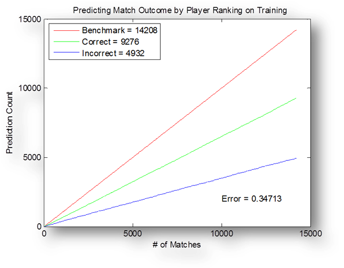
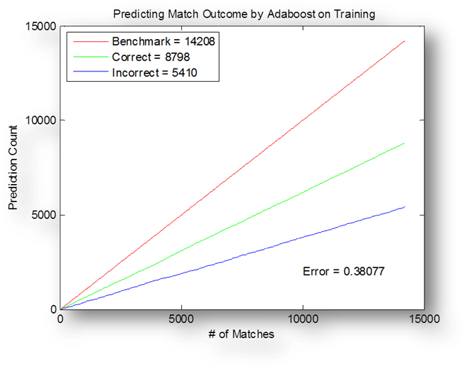
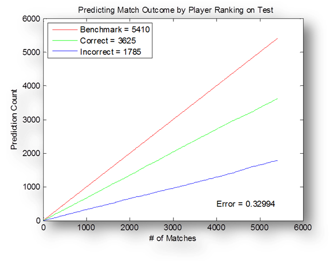
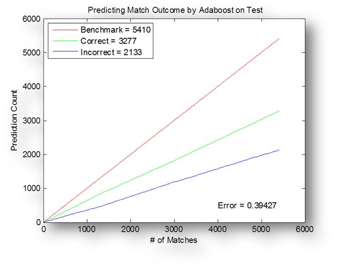
The
training set is composed of 14208 matches and the test set is composed of 5410
matches. A win for the first player is considered a 1,
a win for the second player is considered a 0 in terms of classification.
Top
graph details an attempt to predict match outcome in the training set by
picking the higher ranked player. Expectedly, the error increases as the number
of matches considered increases. Bottom graph details the number of correct
predictions made by Adaboost on the training
set. It is notable that the error is
actually higher than the case of just picking through ranking.
Similar
cases as the above can be seen in the experiments on the test set. Ranking
still outperforms AdaBoost. It seems ranking gives a
nearly 2/3 chance of predicting the correct outcome, while Adaboost
is closer to 60%.
Now,
one of the problems with the training and test sets is that they contain
matches where the ranking difference is massive, on the order of 100. I would
venture to guess that the higher ranked player wins these lopsided matches
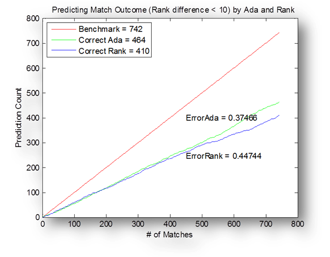
almost all the time. To paint a better visualization of the data, I reduced the
test set to only contain matches where the ranking difference was less than 10.
This reduced the number of examples to 742. Now, ranking only has approximately
55% accuracy, barely better than random guessing whereas Adaboost
still maintains near 60% consistency. It goes without saying that when the
ranking difference is smaller, other factors, such as the ones in the feature
vector, carry more weight.
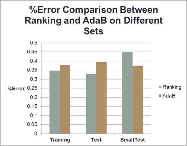
For
the sake of visualization, this bar graph plots the error rates of each method
side by side on the 3 sets.
Problems and Future
So,
there were some errors in my implementation.
1. For the final project, I need to include the ranking data as part of my feature vector. It is valuable data, that cannot just be discarded when creating the feature vector, since it does play such a huge role in everything from the tournament draw to a player's mental state. The goal is to see how the combination of the current features with the rank included will perform with respect to each individually.
2. This brings up another point. I have no way to measure a player's confidence level. Tennis is at its heart a very mental game. Djokovic's tear through 2011 is largely attributed to both his physical and mental strength gain over the off season. In some ways, the previous year's win loss record makes an attempt to capture this, but it is too hard to quantify in a meaningful way.
3. My AdaBoost algorithm was not as efficient as it could have been. In the case of the weak classifiers, I had merely considered the value of the feature in the proximity of zero. That is, if the value of a feature was negative, i.e. the second player had the advantage w.r.t. that feature, I classified the match as a 0. If the value of the feature was positive, i.e. the first player had the advantage w.r.t. that feature, I classified the match as a 1 (a win for the first player). This goes against the point of Adaboost, which should learn the threshold level at which the feature value becomes statistically significant. For improved performance, I will certainly have to go back and implement this.
4.
By
5/20: I seek to have correctly implemented AdaBoost.
By
5/25: I seek to have used one of the methods we have discussed in class and
modify it to classify this problem. Logistic regression is a safe bet.
By
5/28: Compared the results produced by the different methods: ranking, AdaBoost, logistic regression? Final touches and create
poster.
5/30:
Present finished project.
References
[1] https://en.wikipedia.org/wiki/Tennis
[2] https://en.wikipedia.org/wiki/Machine_learning_algorithms
[3] Hamadani Babak. Predicting the outcome of NFL games using machine learning. Project report for Machine Learning, Stanford University.
[4] R.P. Adams,
G.E. Dahl, and I. Murray. Incorporating Side
Information in Probabilistic Matrix Factorization with Gaussian Processes.
Proceedings of the 26th
Conference on Uncertainty in Artificial Intelligence, 2010.
[5] G. Donaker. Applying Machine Learning to MLB
Prediction & Analysis. Project report for CS229 -
Stanford Learning 2005.
[6] J. Matas, J. Sochman. AdaBoost.
Centre for Machine Perception, Czech Technical University, Prague. http://cmp.felk.cvut.cz
[7] Y. Freund,
R.E. Schapire. A Short Introduction
to Boosting, AT&T Labs - Research, Shannon Laboratory. Florham Park,
NJ, 1999.