Scaling up Deep Networks

Introduction

Deep Networks are a up-and-coming machine learning technology. Just several weeks ago, Android's NN voice recognition made the homepage of Wired, and Deep Learning research has made it into the NY Times and the New Yorker. A Deep Network, in the simplest sense, is a multi-layered Neural Network. These have shown to be effective, but unfortunately very time consuming to train. Our goal was to use the power of parallel programming to speed up the training of a neural net. To do this, we had a sequentially trained neural net that we used as a control, and compared this to the performance of a parallelized training algorithm we developed called ScatterBrain.

Neural Network and Dataset

We used a simple data set, allowing us to run many time trials. The data set comes from UC Irvine Machine Learning Repository [7] and models the state of the shuttle during takeoff. There are 9 numerical inputs, an integer output value from 1-7, and 43500 instances. We converted the input to values between 0 and 1, and the output into seven nodes, with values 0 or 1. We tuned the hyperparameters of the sequential Neural Net and found that 3 hidden layers with 8 nodes each, and a learning rate of 0.3 worked very well, giving accuracy of 99.5%. We used a sigmoid activation function.

ScatterBrain: A Parallelized SGD

Parallelized SGD and the ScatterBrain Algorithm

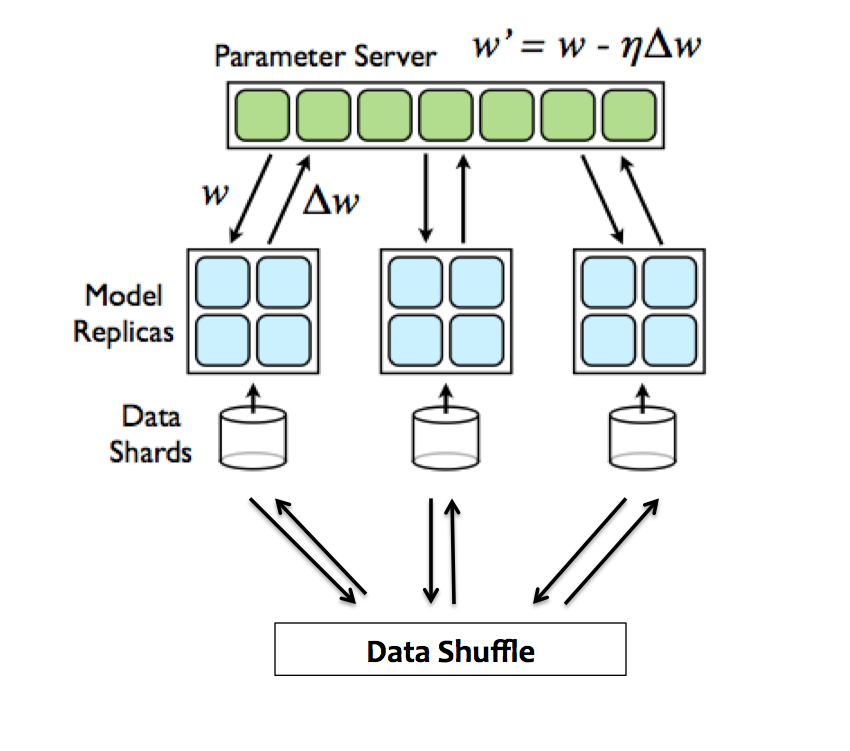
Figure 4. Depiction of the parallel training model, modified from [1].

The parallel model we used on was inspired by work done Dean et al. [1] on what they call Downpour SGD. It takes the inherently sequential training algorithm, SGD, and tries to split up the work. There is a server of parameters (the weights that you are trying to optimize), and a group of clients that are all individually running SGD on data shards. Periodically, the clients tell the server what changes they've made to the parameters. The server takes the updates, and updates its master copy of the parameters. The clients also periodically request the parameters from the server, and the servers sends that client the master copy. The clients all run asynchronously, so there doesn't need to be any communication between them. Only the parameters and updates need to be broadcasted, and only between the server and clients. Notice that the clients are not necessarily always running with the most recent set of parameters. They might run SGD and find updates on an outdated copy. This introduces another degree of randomness, that the original researchers actually found to be very benefical for keeping the model out of local minima.

Our implementation had some simplifications and modifications to Downpour SGD. While Downpour SGD assumes that the clients are individually running a complex parallel SGD framework called Distbelief, our data set was small enough to remain in the memory of each client and we opted to run a simple SGD on each client. Similarly, our parameter server is simply one core, versus the multicore version presented in [1]. Because we were consistent in the form of SGD that the sequential version and the parallelized version use, this still provides a excellent platform on which to compare the effect of the parallel division of SGD. The other modification we made was to shuffle the data amongst the data shards several times during the course of the algorithm; we found that this allows for quicker convergence as it allows for each client to use more data in its descent. We also used a constant scaling between client updates and server updates. Downpour uses a different scaling for every parameter, but we found our data set didn't require such tuning, so we opted for a simple constant step size. With these changes Downpour SGD morphed into ScatterBrain!

Theoretical Speed Up

A standard measure of the degree of parallelism one can achieve with an algorithm is speedup. Speedup is the ratio between the amount of time it takes to complete a task on one processor and the amount of time it takes to complete that task with p processors. An ideal speedup is linear speedup, where the value is p. In this case, assuming a sufficiently large input such that each processor has something to do, the more processors you have the faster the computation is, with no upper ceiling.

SGD iterates over all the examples in the training set of size s, calculates the error for each, and then updates the parameters. In the parallel implementation with p processors, however, it runs a standard SGD over a training set of s/p. As discussed previously, ScatterBrain isn't totally equivalent to SGD, which depends on the parameters of the previous iterations (an inherently sequential operation). However, ScatterBrain still converges on a minimum, and we expect it to do so at a rate similar to the sequential case, aside from a little more noise. This therefore gives us linear speedup, and indicates that it is a prime candidate for parallelization.

Implementation

To actually implement this algorithm, we investigated several parallel programming paradigms: CILK, CUDA C, and MPI.

Cilk is a programming language, very similar to ANSI C, with several keywords that fork the program into parallel processes into seperate threads and later sync them back together. Although this would be simple to implement, Cilk is designed for Symmetric Multiprocessors, which all have access to a single main memory. With the ultimate goal of making the parallel SGD scalable, this would be problematic, because the whole data set would NOT neccessarily fit on a single main memory.

Another common approach, widely researched, is the use of a GPU. A GPU is the graphics card on a computer, and it has an architecture consisting of a large number of multiprocessors. Additionally, nVidia has a language similar to C, called CUDA C, which can be used to program their GPU's. This gives us a highly parallel architecture to use. However, once again, scalability becomes a problem because GPU's have severe memory limitations (6 GB) and don't communicate between each other easily or well.

Lastly, we have MPI (Message Passing Interface), which is a communication protocol with an implementation as a library in C. MPI provides communication functionality between a set of processes, each which has been mapped to a node in a cluster. Since MPI revolves around broadcasting and recieving data like the algorithm we are using, and each process is mapped to a node with its own memory, MPI fits our problem intuitively and is open to massive scalability.

Ultimately, MPI ended up being a great choice. MPI-2, a somewhat newer extension of MPI, offers one-sided communication capabilities. One-sided communications are named as such because only one process needs to issue a send or receive call to achieve the communication, as opposed to having both sides exchange SEND and RECIEVE calls. This is perfect for our algorithm, where what is stored on a central parameter server is essentially treated as shared memory by all the clients, with explicit communication abstracted away.

Pseudocode

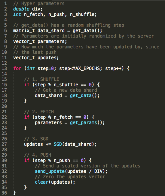
Figure 5. Our pseudocoded algorithm.

Here is the specific pseudocode for ScatterBrain. The main things to note is the fetching and pushing of parameters (lines 22 and 30). Also note the data shuffling and scaling of the pushed parameter update. In between those two operations is a typical SGD, that closely resembles what we used earlier in the sequential case. We are particularly excited about how generalizable this algorithm is; it makes no distinction between regular Neural Nets and Deep Nets, or even the use of an ANN at all. We expect that this will be similarly effective for any algorithm that uses Stochastic Gradient Descent.

Results

Tuning Hyperparameters

ScatterBrain introduced a number of new hyperparameters - the n_fetch, n_push and n_shuffle values, as well as DIV and the number of clients. We initially tested values of n_fetch and n_push that were equal, and found that they could go as high as 300 without sacrificing performance (for reference, we capped the number of epochs at 5000, and typical runs last up to 1500). This might be due to a particularly uniform data set, giving rise to similar data shards. We then varied n_fetch and n_push so that they were not equal. Variations of a few dozen steps didn't cause a change in performance. We were also able to increase the push rate a factor of 10 above the fetch rate with good results. But increasing the fetch rate above the push rate gave terrible performance -- it couldn't converge and would run for the maximum number of epochs. This is because the server was being rarely updated, but clients were continually fetching the same parameters and thus being reset back to their starting points.

Below are some plots of the hyperparameter analysis for DIV, n_shuffle and the number of processors.

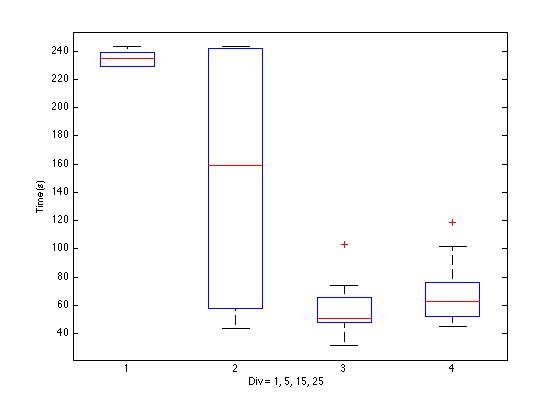
Figure 5. Effect of changing the DIV value. In the first case, DIV=1, the gradient descent was failing to converge and maxed out the number of iterations. In the second case, performace was sometimes acceptable, but sometimes it would also fail to converge and run for the maximum possible time. Hence the high standard deviation. DIV=15, or the number of clients, is clearly optimal. Higher values give similar error performance, but take longer to converge because steps are smaller.

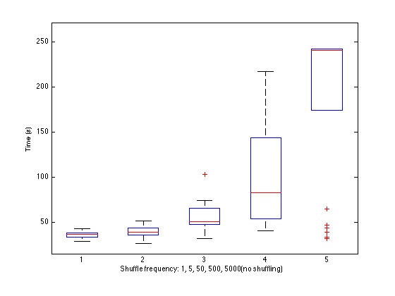
Figure 5. Effect of changing the n_shuffle value. Without shuffling, the last case, fast processors end early and take their data shards out of circulation. Slower processors then fail to converge, maxing out the allowed number of epochs, and leading to higher average time. Our data set is so small that we don't see the cost trade-off of performing more shuffling steps, so more shuffling leads to better averages and deviations. We expect that this would scale very poorly with larger data sets. Fortunately, shuffling only once or twice (n_shuffle=500) appears to still have a very beneficial effect.

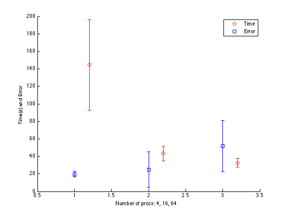
Figure 5. Effect of using different number of processors. This result is tied very closely to our particular data set, but shows a trend that makes intuitive sense. With fewer processors, there is less paralization and thus higher time. But conversely, when you split up the data shards too small, clients struggle to agree on overall minima and error is higher. It thus becomes a balance between time and desired error performance.

Analysing the Descent

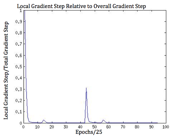
Figure 5. Our pseudocoded algorithm.

To investigate how the algorithm navigated the parameter space, we plotted the ratio of the magnitude of a single "watchdog" clients parameter update to the magnitude of overall parameter updates accumulated over a time slice of 25 epochs. We sampled every 25 epochs to see how this changed over the course of the algorithm. The values of this ratio tended to be very small, indicating either that the clients descend in roughly the same direction or that client didn't move much over the time slice because of a local minium. The latter is unlikely, because the movements of the other clients would bump it out of the minimum. It is also interesting to note that there are several spikes in this plot, indicating either that the "watchdog" client has a particularly steep gradient relative to the others or that there is local miniumum and several of the clients provide updates that cancel each other out. Because we are measuring over a time slice of 25 epochs, the former is unlikely if the data shards all have similar distributions. Notice that even in these spikes, the value of the measurement does not get larger than one, indicating that the Descent is still continuing in a rougly uniform direction even if some of the clients get caught up in local minima.

Final Results

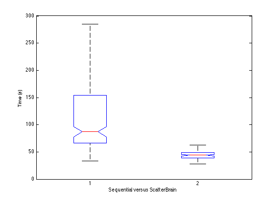
Figure 5. Final time analysis: Sequential versus ScatterBrain.

The ScatterBrain algorithm was about 60% faster than traditional SGD on average using 16 cores, DIV=15, n_fetch = n_push = 300 and n_shuffle = 15. It also has much less variability in time to completion. However, this still much slower than the predicted 16x(linear speedup). This is likely because there is overhead in the communications process, which takes constant time. On small datasets, as we were using, this constant overhead is relatively significant. However as the problem size increases, the constant time becomes relatively smaller (although costly communications like shuffling would be more costly). The paralized SGD is also not completely equivalent to the sequential version, so linear speed up is certainly a "best case" scenario. Still, the increases in efficincy are tangible even on a small dataset with about 30,000 training instances.

Further Work

We have ascertained that the ScatterBrain algorithm effectively parallelizes SGD, but we have only trained and tested ANN's using this method on very small datasets of about 45,000 instances, which would easily be handled by sequential code. Further work should include using and training deeper ANN's using the ScatterBrain on massive data sets, where operations such as shuffling could be very expensive and time-consuming. We would also like to investigate the possibility of using overlapping data shards, which may help eliminate the need for shuffle operations. And finally, in this comparison, the clients were running a very simple version of SGD. The clients can, and should, be further optimized individually to help performance as the data set increases. Fortunately, the framework that ScatterBrain developes is simple enough that introducing such changes are easily made.

References:

External Software

All the code was developed by us, though parts of the sequential neural net were originally modelled after a toy online sample in C# and subsequently heavily modified. The code snippet used is towards the bottom of the following page:

Other References