Face Betrays Your Age

Xin Wang, Yanan Li, Yongfu Lou

Abstract

Even though relatively limited efforts have been made towards it, age estimation has a large variety of applications ranging from access control, human machine interaction, person identification and data mining and organization. Human face is the most essential reflection of age. During the process of aging, changes of face shape and texture will take place.

This project is about estimating human age based on face images. It was split into four stages: dataset obtaining and preprocessing, shape and texture feature extraction, model training and age prediction, comparing prediction errors of deferent models.

Dataset

The database we are used is FG-NET(Face and Gesture Recognition Research Network), which is built by the group of European Union project FG-NET. This dataset contains 1002 images of 82 subjects whose age varies from 0 to 69. Each image was manually annotated with 68 landmark points located on the face. And for each image, the corresponding points file is available. Figure 1 is a sample image from the dataset.

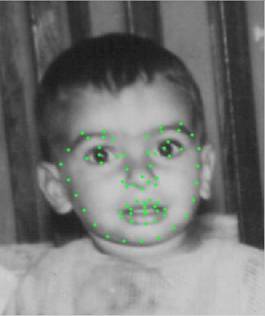
Figure 1. Image sample from the dataset

Data Preprocessing

Phase 1: Filtering

To simplify the processing and enhance the prediction accuracy by the end, we chose only the images in which people roughly faced the camera directly. Images like Figure 2 were not chosen. At last, we got 617 satisfying images out of the total 1002 images in the dataset.

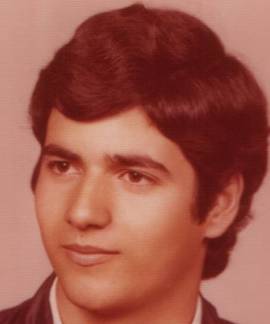
Figure 2. Image sample not chosen

Phase 2. Graying

Since we need to use the texture on the face as one important feature that predicts the age, we processed all the images into gray scale ones.

Phase 3. Rotation

Each image was rotated until the two eyes reached horizontal.

Phase 4. Resizing

We resized all the images. Go through all the coordinates files to find the shortest distance D between two eyes in each image and then resize all the images until the eye-distance in each image is equal to D.

The whole procedure of data preprocessing is shown as Figure 3.

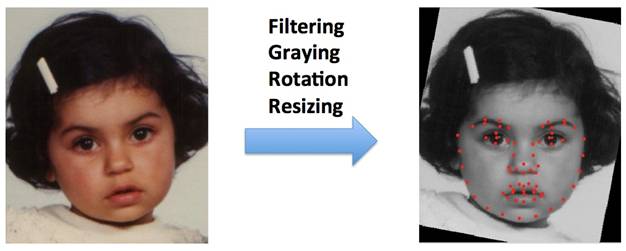
Figure 3. Procedure of data preprocessing

Feature Extraction

1.Shape Feature vectors obtained from Shape Model

A. After the data preprocessing stage, we have 617 images and the corresponding coordinate files, with each one recording 68 point-positions on the face.

B. We aligned the shape vectors a little further by applying depth angle modification to make the people exactly face the camera directly. Figure 4 shows the procedure.

The new shape vector we got can be presented as following:

C. Reduce the dimension of the shape vector to accelerate the model training procedure later by using Principle Component Analysis.

PCA is applied to the shape vector by computing the mean shape:

And the covariance,

The eigenvalues and eigenvectors of the covariance matrix, epresents for the eigenvalues, and is listed in descending order.

Choose the t largest eigenvalues which can explain the 98% of the variance in the training shapes.

So we can get eigenvalues , and the corresponding eigenvectors.

After PCA, each shape vector can be written as a linear combination of and:

In the above formula,, which are the shape parameters and the coefficients of the first t models.

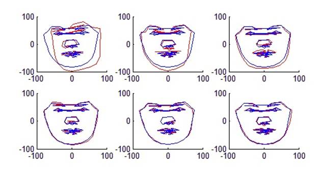
Figure 4. Mean face shape and some eigenvector variations

(Blue lines show the mean shape and red lines show some eigenvector variations based on the mean shape )

2. Texture Feature vectors obtained from Appearance Model.

To establish the statistical texture model for reflecting the global texture variation of the faces, firstly, what we need to do is getting all the pixel gray-scale values in the face contour area, which can be regarded as extracting the shape-independent texture. And then we use principle component analysis of the shape-independent texture to modeling.

A. Texture normalization

Texture normalization is used to compensate the illumination difference in all the images. We need to get the grey-scale value of each pixel in the texture image in a fixed sequence to generate a vector where n is the number of the pixels. And the elements in this vector have a mean of 0 and a variance of 1.

B. Triangulation of the mean shape

We introduced Delaunay Triangulation method to divide the mean shape into a collection of triangles (triangular meshes).

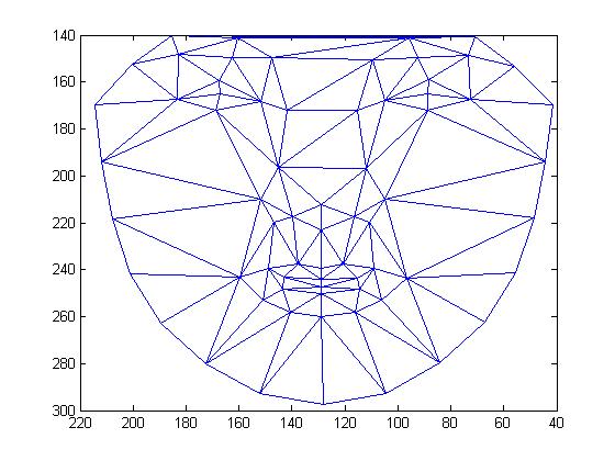
Figure 5. Delaunay Triangulation of the mean shape

C. Obtaining the shape-independent texture.

Firstly, each training image is deformed into the mean shape image by piecewise affine transformation. After that, we will find that there are some black lines in the new image which are 0 pixels. To fill all the blank pixels (value=0) generated by the affine transformation, interpolation on the deformed image is applied. Then, the shape-independent texture feature is generated.

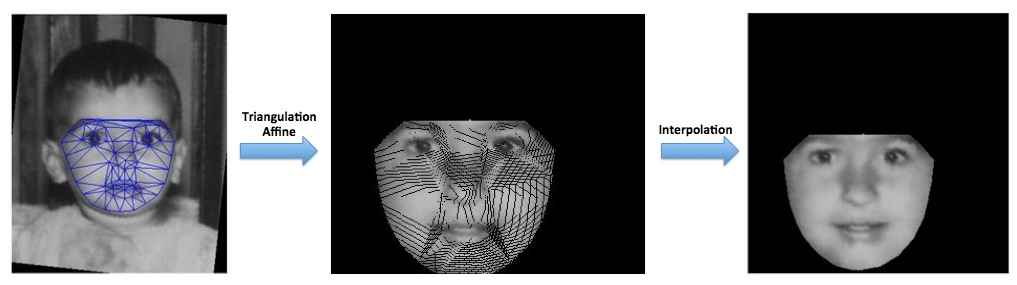
Figure 6. The procedure to obtain shape-independent texture

D. Principle Components Analysis.

Like shape feature extraction, AAM also use principle component analysis to build a statistical model of texture. As a result, we can get the eigenvalues, eigenvectors and the mean texture of the appearance model, and after PCA, each shape vector can be written as a linear combination of mean texture and the eigenvectors.

Till now, we have all the needed feature vectors, shape and texture. In the next stage, SVC and SVR are used to train a model and estimate ages. For SVR, there are two execution plans. The first is to use the combined shape and texture vectors which are dimension-reduced again by applying PCA. The other is to use hierarchical SVRs with the two separate features.

Training Models

In this stage we applied four models, and made comparisons of the results.

Model 1: SVC (Support Vector Classification)

The SVC method in this project is C-SVC. Using the combined shape and texture feature vectors, we built 18 different models according to the class size. They are 1-year-a-class, 2-year-a-class, ... , 18-year-a-class respectively. And at last, we calculated and compared the standard error of the models trying to find the best class size.

Model 2: SVR (Support Vector Regression)

Specifically, what we used is epsilon-SVR, one kind of SVR. In this model, the shape feature vectors and the texture feature vectors are also combined to form the overall feature vectors. These vectors are then used to train the model.

Model 3: Hierarchical SVC

Before we use SVC or SVR to train the model, we have 2 kinds of features, shape features and texture features. They are combined in the above two models. However, different kinds of features usually have distinct magnitudes. The features with lower magnitude will be assigned lower weight in SVM, thus relatively neglected. They didn’t get the deserved influence on the result, which leads to the higher inaccuracy of the result.

Therefore, we introduce Hierarchical SVM which was suggested by Professor Lorenzo. Hierarchical Support Vector Machine (HSVM) for multi-class classification is a decision tree with an SVM at each node. In this model, we used three SVC models at each node. The first SVC was trained using only the shape feature vectors and the second using only the texture feature vectors. We got two prediction result vectors and then combined them (prediction from the first SVC, the second SVC and the labels) as the new feature vectors. At last, we trained a third SVC using the above feature vectors. And the prediction procedure of the new model is shown in Figure 7.

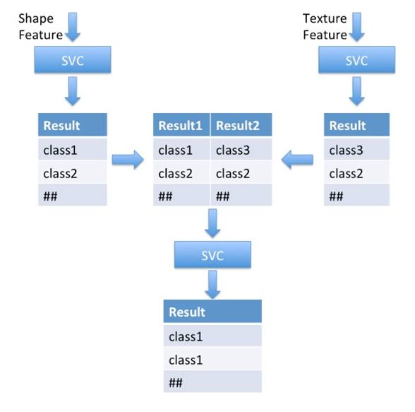
Figure 7. Prediction process unsing Hierarchical SVC

Moreover, Hierarchical models are better for large amount of data. The number of levels should be controlled in some degree, since if there are too many levels, data may not be enough to train a model well and the way from root to leaf maybe too long to make it right to the correct leaf.

Further, we can use multi-level Hierarchical SVM instead of 2 levels. On each node, SVM can have different parameters, we can choose the optical parameter depend on the result from the previous level.

Model 4: Hierarchical SVR

Hierarchical SVR is very similar to hierarchical SVC and the difference between them is that in the first model we used three SVCs while second one we used three SVR nodes.

Experiments and Results

Ÿ Result for C-SVC

Figure 8 shows the classification accuracy as a function of class size.

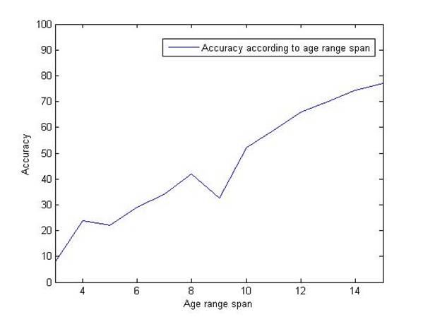
Figure 8. Classification accuracy of C-SVC

Ÿ Result for Hierarchical C-SVC

Figure 9 shows the classification accuracy as a function of class size.

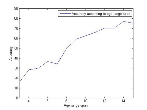
Figure 9. Classification accuracy of Hierarchical C-SVC

After implementing hierarchical model to SVC, a light improvement appears. Later we can observe a larger performance improvement when SVR is optimized by hierarchical model.

Another important thought suggested by the professor is the standard error of SVC should go down then come up. Because if age span is small, there are not enough samples to train the model. While if the age span is large, then the error is big, this is caused by precision itself. By observing the standard error of different age-span, we can make a balance of training maturity and precision, thus find the best age-span. From the following plot, the best age-span can be chosen, which is 14 year.

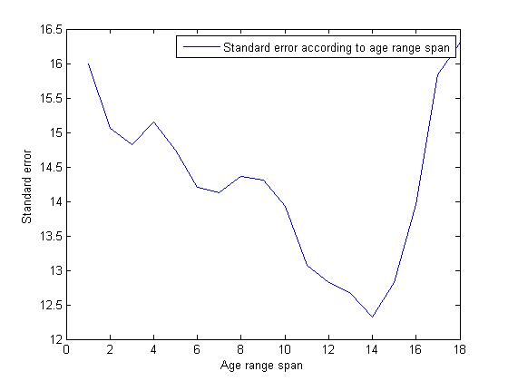
Figure 10. Classification standard error of Hierarchical C-SVC

Ÿ Result for Epsilon-SVR and Hierarchical Epsilon-SVR

Figure 10 shows the mean squared errors and other parameters of SVR and Hierarchical SVR.

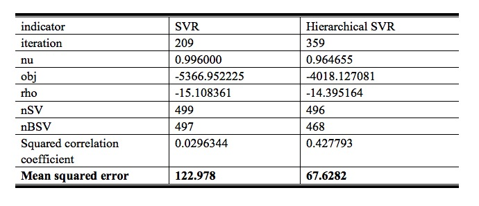
Figure 11. Mean squared errors of SVR and Hierarchical SVR

From the results, we can generally get some conclusions:

a. Accuracy gets higher when age range span grows. The standard error goes down and rises, which can be used to decide the best class age-span.

b. Hierarchical SVR and SVC performs better than normal ones. The reason has been stated in the part of hierarchical models.

c. SVR produces smaller error than SVC.

When we compare the SVC and SVR, we cannot regard SVR as a fine-grained SVC. If so, SVR will have the lowest accuracy. It was the opposite because of an assumption that all misclassifications are equal, SVC missed a very informative part of the data, therefore is not as good as SVR in this problem.

Summary

Facial age estimation can figure in a variety of applications. However, it is quite challenging a task. In this project, we proposed an age estimation method. Firstly, shape and texture features are extracted from the faces. Then we train four different models and predict human ages using them. After analysis and comparison on the results (for SVC is the misclassification rate and for SVR is the mean square error), we can conclude that the whole process produces a quite acceptable overall result.

External Software Modified

There are mainly two sections we use the external code. The first one is AAM&ASM for feature extraction and the second is SVM algorithms for model training. Original Code, sources of external software and how we modified them by writing own code are listed as following.

	Data preprocessing	AAM&ASM	SVM
External Source Link		Active Appearance Model and Active Appearance Model http://www.mathworks.com/matlabcentral/fileexchange/26706-active-shape-model-asm-and-active-appearance-model-aam By Dirk-Jan Kroon	libsvm http://www.csie.ntu.edu.tw/~cjlin/libsvm/ By Chih-Chung Chang and Chih-Jen Lin
Code Written by Own	1. dataPreprocess.m: Data Preprocessing procedure including reading the coordinates, image, identifier and age, storing them in a structure, change all the images into gray-scale ones, applying rotation to the coordinates and the image, applying scaling to the coordinates and the image and applying depth angle modification to the coordinate and the images. 2. makelabel.m: Make labels for classes with different age range. 3. showImgPnt.m: Show the visualization of feature points on a picture after data Preprocessing.	The basic idea of the project we refer is to train Active Shape Model and Active Appearance Model for automatic segmentation and recognition of biomedical objects. However, our project is to extract feature from the training set and the 68 landmarks are already known. So we modified the source code and we neglect the search step and add piecewise affine transformation in it. 1. average_shape.m: Calculate the mean face shape of the original data. 2. triangulation.m: Apply Delaunay Triangulation to get the triangular meshes of mean shape. 3. triangleAffine.m: Apply piecewise affine transformation to deform each face into mean shape. 4. GetShapeFeature.m: Get the shape feature vector of the training data. 5. GetAppearanceFeature.m: Get the texture feature vector of the training data. 6. GetCombinedFeature.m: Get the combined shape and appearance feature vectors of the training data. 7. PCA.m: Reduce the dimension of the feature vectors to accelerate the model training and age prediction processes.	1. combineData.m: Combine the output data files obtained from feature extraction stage. 2. SVC.m: Using SVC to predict people's age. 3. SVR.m: Using SVR to predict people's age. 4. hSVC.m: Using hierarchical SVC to predict people's age. 5. hSVR.m: Using hierarchical SVR to predict people's age. 6. DifRangeSVC.m: To plot the accuracy as a function of class size. 7. DifRangeHSVC.m: To plot the accuracy as a function of class size.

Table 1. Original Code and External code modification details

References

[1] Xin Geng, Zhi-Hua Zhou, Kate Smith-Miles (2007). Automatic Age Estimation Based on Facial Aging Patterns. Pattern Analysis Machine Intelligence, 29(12), 2234-2240.

[2] Unsang Park, Yiying Tong, Anil K.Jain (2010). Age-Ivariant Face Recognition. Pattern Analysis and Machine Intelligence, 32(5), 947-954.

[3] Ramanathan, N., Chellappa, R., & Biswas, S. (2009). Age progression in human faces: A survey. Visual Languages and Computing.

[4] Steiner, M. Facial Image-based Age Estimation.

[5] Xing Gao. Research on Facial Image Age Estimation.

[6] Hsu, C. W., Chang, C. C., & Lin, C. J. (2009). A practical guide to support vector classification, 2003. Paper available at http://www. csie. ntu. edu. tw/~cjlin/papers/guide/guide. pdf.

[7] Van Ginneken, B., Frangi, A. F., Staal, J. J., ter Haar Romeny, B. M., & Viergever, M. A. (2002). Active shape model segmentation with optimal features. Medical Imaging, IEEE Transactions on, 21(8), 924-933.

[8] Cootes, T. F., Taylor, C. J., Cooper, D. H., & Graham, J. (1995). Active shape models-their training and application. Computer vision and image understanding, 61(1), 38-59.

[9] Cootes, T. F., Edwards, G. J., & Taylor, C. J. (2001). Active appearance models. Pattern Analysis and Machine Intelligence, IEEE Transactions on, 23(6), 681-685.

[10] Chih-Chung Chang and Chih-Jen Lin, LIBSVM : a library for support vector machines. ACM Transactions on Intelligent Systems and Technology, 2:27:1--27:27, 2011. Software available at http://www.csie.ntu.edu.tw/~cjlin/libsvm