Background
Meteorologists still lack the ability to produce truly accurate weather forecasts, especially with respect to precipitation. Nature's complex phenomena and the scope of the problem in both time and space leads to predictions that sometimes vary greatly from the actual weather experienced (Santhanam et all, 2011). Figure 1 (HPC,2012) is provided by the National Oceanic and Atmospheric Administration (NOAA) and demonstrates the accuracy of quantitative precipitation forecasts from three different prediction models. the North American Mesoscale (NAM), the Global Forecast System (GFS), and the Hydrometeorological Prediction Center (HPC). A threat score is a function that ranges from 0 to 1 and provides a measure of how good a prediction was, with 1 being a perfect prediction. These inaccurate predictions provide good motivation for developing a better precipitation prediction algorithm.
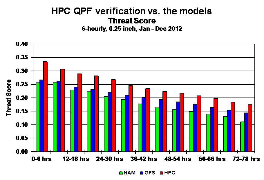
Figure 1
Updated Problem and Scope
Our original goal was to predict snow in Hanover, NH 24 hours in advance. The data we found and are using however, turned out to be strictly in terms of hourly precipitation, and not in terms of accumulated snowfall. There was data on total snow coverage in kg/m^2 available, which obviously accounted for falling snow, but it also accounted for melting snow, ground temperature, etc. Because of this, we found it to be an inaccurate measure of how much snow accumulated due to a storm front, and chose to use the precipitation data for our project instead. We can still determine snow from rain based on ambient ground temperature, one of our input variables. We cannot however know the amount of snow which fell due to unknown variations in snow water density. While we can still focus on predicting snowfall, the prediction problem is entirely focused on precipitation. We will use ground surface temperature as an indicator of snow or rain but we will still consider all precipitation events in our data set during training.
Our goal at the start was to predict the probability of snowfall in Hanover 24 hours in advance. However, due to our recent struggles to get an accurate predictor we may reduce the prediction timeframe to only 6 hours in advance, as will be discussed later. After obtaining successful results in the 6-hour timeframe, we will try to increase the interval, ideally reaching a full day. We plan on making our prediction using a feed forward neural network which will output the posterior probability of precipitation given the input variables.
Data
All of our data was obtained from the Physical Sciences Division of the National Oceanic and Atmospheric Administration. Which weather variables are most relevant to snowfall and the physical distance of measurements from Hanover necessary to predict snowfall was determined through an interview with a meteorology Ph.D. candidate at the University of Utah. We concluded that on the earth's surface we should consider wind direction, relative humidity, and mean sea level pressure. At elevations (measured in pressure) 500mb, 700mb, and 850mb we should use wind direction, relative humidity, specific humidity and geopotential height. For these variables, predicting precipitation one day in advance can depend on variables up to and over 1,000 miles away. Thus we selected the location of measurements for our data to approximate a box surrounding Hanover of approximately 2,000 miles in width and height. Figure 2 shows this box, with the blue marker indicating the location of Hanover and red markers representing the location of variable measurements.
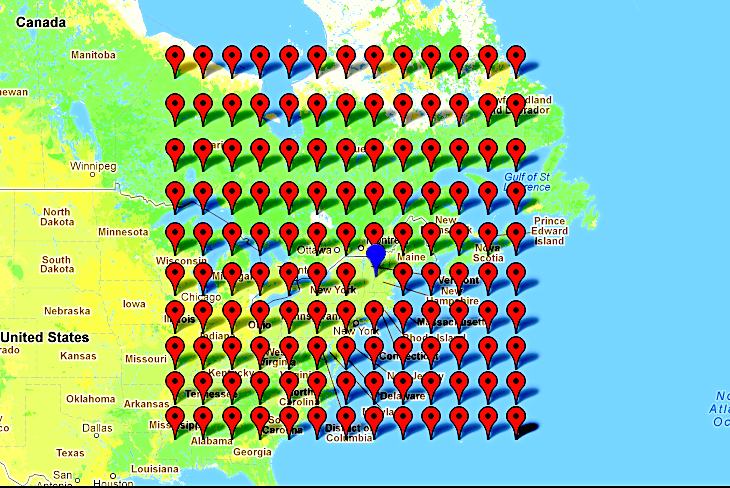
Figure 2
Once our source was selected, the first step in obtaining data was to download the files (~50GB) and reformat them. The data was separated by variable and year, and formatted in .netCdf files, with one file corresponding to one year for one variable. Due to variable measurements spanning 1948-2001 on a 6-hour time interval and precipitation measurements in Hanover spanning 1979-present on hourly intervals, we had to choose the overlapping period for our training data. This provided us with a total of 23 years of training data separated over 6-hour intervals, which corresponds to 33,600 individual samples. Using a 13x10 grid of measurements for our 19 variables of choice (four on the surface, five at three different pressure levels) gave 2,470 input variables.
Once the .netCdf files were downloaded, we extracted the 3-dimensional matrix of measurements for each variable over the time frame and geographical spread in which we are interested. These matrices had dimensions corresponding to latitude, longitude and time, with measurements for one year, or 1,460 (1,464 for a leap year) 6-hour time intervals. However, because we are considering each location of a variable's measurement to be a distinct feature in our algorithm, each of these matrices had one year of measurements for 130 different features. For our training data, we then transformed and combined these matrices into 2-dimensional matrices with rows corresponding to time intervals, and columns to features. Each of these matrices corresponded to one year, and were thus size 1,460x2,470 (1,464x2,470 for a leap year). When doing this we also reindexed the precipitation for each year so that the ith row of the precipitation vector was 'n' 6-hour intervals ahead of the ith row of our feature training matrix, where '6n' is the length ahead of time that we want to make our prediction. Our first training set was designed for a 24-hour prediction time. After failing to generate results, however, we created another training set for a 6-hour prediction time to try and generate results within a smaller timeframe first.
Once we had training matrices for each year, we normalized each input variable independently to ensure that no single variable's magnitude was disproportionate to its relative importance. Specifically, for each value of a given variable, we subtracted the variable's mean and divided by the standard deviation. These recalculated variable values then have a zero mean and unit standard deviation over the entire data set. In order to attempt both classification and regression algorithms, we also created two different precipitation vectors for training data. One vector has the real-valued amount of precipitation in inches over the given time interval, and the other has boolean values, where y=1 if there was precipitation in the given time interval and y=0 otherwise.
Algorithms
Neural Network
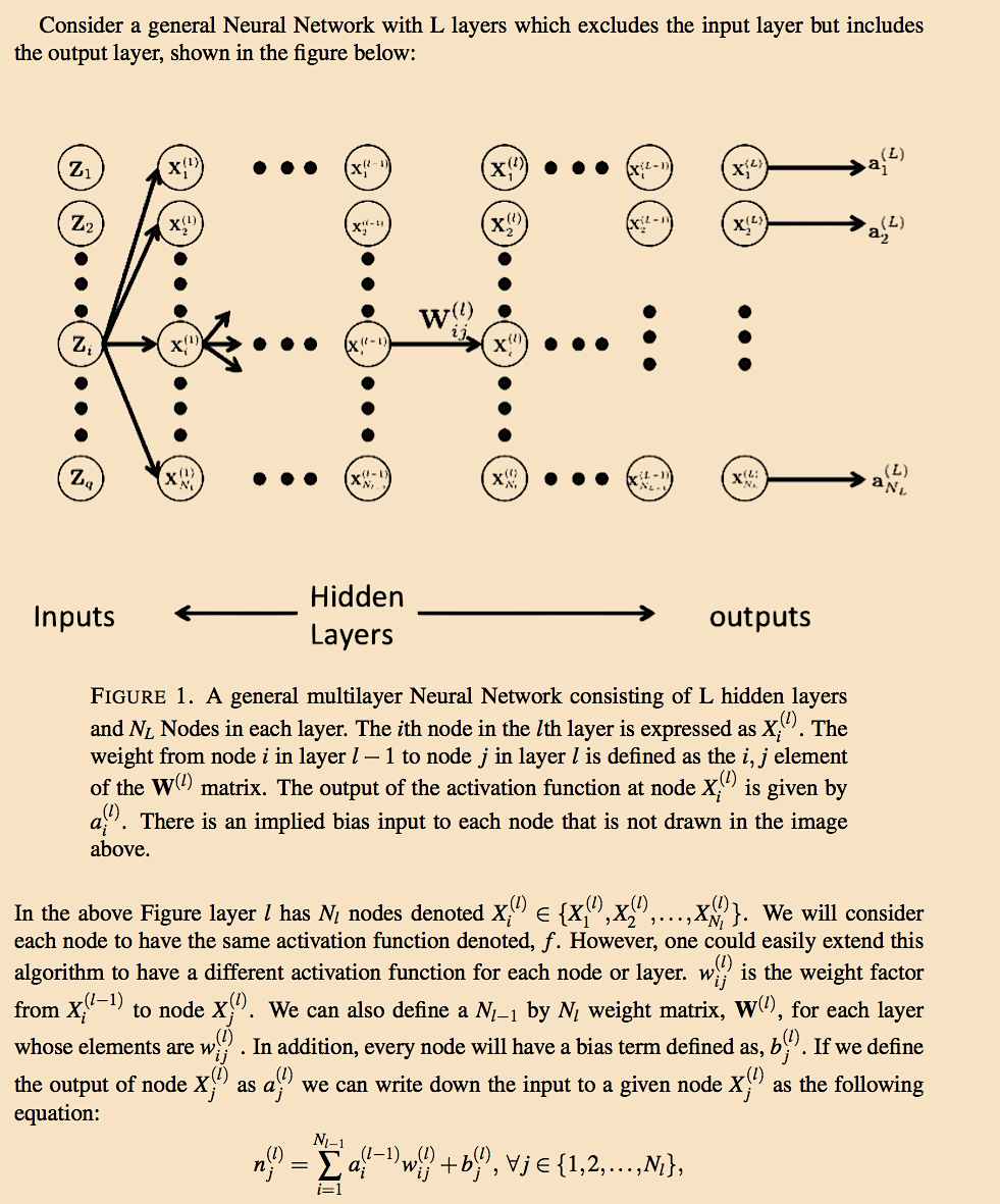
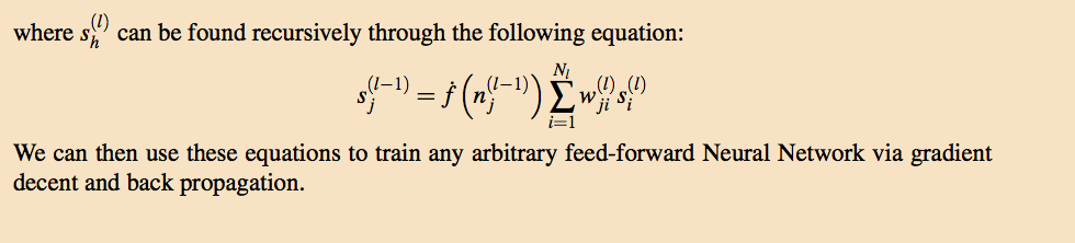
We have implemented a feed-forward back propagation neural network. The structure of the network has been generalized to allow for any number of hidden layers with any number of nodes in each layer. This means we have several hyper parameters that need to be tuned, such as the number of hidden layers and the number of nodes on each layer. The structure of the network can be seen in the figure below. Networks with only two hidden layers have been shown to be able to model any continuous function with arbitrary precision. With three or more hidden layers these networks can generate arbitrary decision boundaries (Bishop, 1995). Furthermore, the output of a neural network for a classification problem has been shown to provide a direct estimate of the posterior probabilities (Zhang, 2000). The ability to model arbitrary decision boundaries is of particular interest for us since since weather phenomena has been shown to be highly non-linear and dependent on large number of variables.
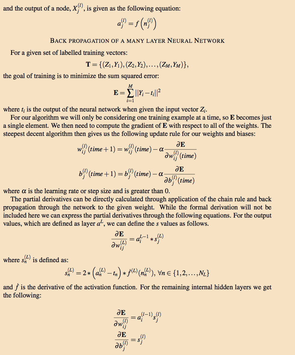
The training of the neural network is done by the generalized back propagation algorithm to optimize the sum squared error as a function of the weights of each node output and the bias values. An exact value for the gradient can be computed through application of the chain rule. Our implementation is a variation of the one outlined by K. Ming Leung in his lecture on Back-propagation in Multilayer perceptrons.(Leung, 2008). The weights are initialized by sampling from a gaussian distribution with a mean of 0 and a variance of the square root of the number of input variables as suggested by Bishop (Bishop, 1995). Below we will discuss the generalized learning rule and methodology for our gradient decent method.
Furthermore, we have worked to improve the training time of the algorithm by randomly choosing a single example from the training set without replacement and updating the weights based on the sum squared error with respect to this training example instead of batch optimization. There is also an optional momentum parameter which will add a fraction of the previous step direction to the current step direction. After all examples have been selected, We evaluate our network over the entire training set. If there is no significant change in the sum squared error then the step size will be reduced and the process repeated.
Since we are only considering one training example at a time, our stopping criteria was set to be based on whether a certain number of consecutive points meet a given threshold or if a maximum number of epochs is reached. All three parameters can be set by the user.
Naive Bayes
The Naive Bayes classifier is based off of the code created for homework assignment 2. This makes the conditional independence assumption of each variable. This is not a particularly valid assumption for our data set since weather between closely separated observation locations will share many similar values, and is unlikely to be independent. As expected, the naive Bayes misclassified every single precipitation event 24 hours ahead of time, clearly making it not an algorithm of choice for our problem.
Random Forest
We also implemented a random forest of decision trees. 11,000,000+ possible splits were generated by sorting each variable and taking the midpoint between any two examples where the boolean output value changed between the two output examples. The forest originally trained each node based on a random subset of 5,000 of the 11,000,000+ possible splits. Unfortunately, when trying to make predictions 24 hours in advance, the random forest produced very few accurate precipitation predictions, misclassifying almost all precipitation events as non-precipitation.
Progress
Thus far we are relatively on course with our proposed dates and progress checkpoints. We have chosen, downloaded, and saved our data in the filetype and format that we need, and written code code for a generic Neural Network, Naive Bayes Classifier, as well as a Decision Tree forest.
For the Neural Network we can define any number of hidden layers as well as nodes per layer. In an attempt to tune these hyper parameters we ran 10-fold cross validation of 10 different network architectures to get a feel for what complexity works best with our model. The 10 cases performed had the same number of nodes in each layer, with the exception of the output layer which is only one node. The number of hidden layers and nodes per layer for each case are as follows: (2,5), (2,10), (2,20), (3,5), (3,10), (3,20), (4,5), (4,10), (4,20). We began by trying to model the quantity of rain 24 hours in the future by attempting to fit the numerical precipitation value. These results can be seen below in Figures 3 and 4. Figure 3 shows our average validation scores of each case as a function of hidden layers and number of nodes per layer. While the results look very good initially, they fail to predict any precipitation events. Due to the fact that there is an overwhelming number of non-precipitation examples. Our model simply learned to send all examples to zero. Figure 4 gives an example of the error during the training of a neural network with 3 hidden layers and 10 nodes per layer. To generate this graph our neural network's performance is evaluated on the entire test and training set every 5000 epochs during the training.
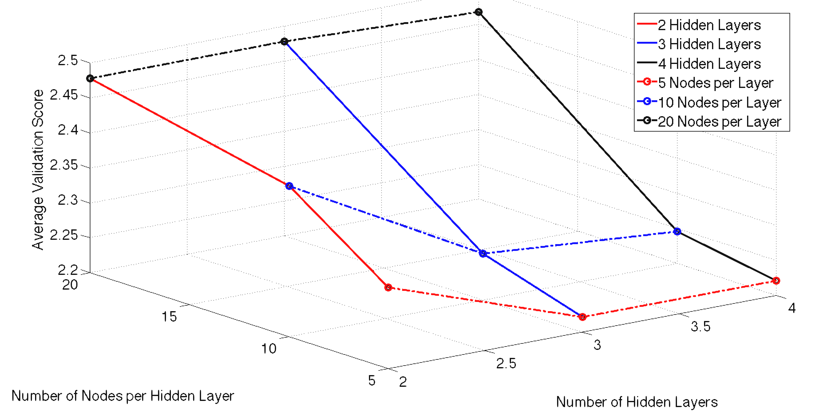
Figure 3
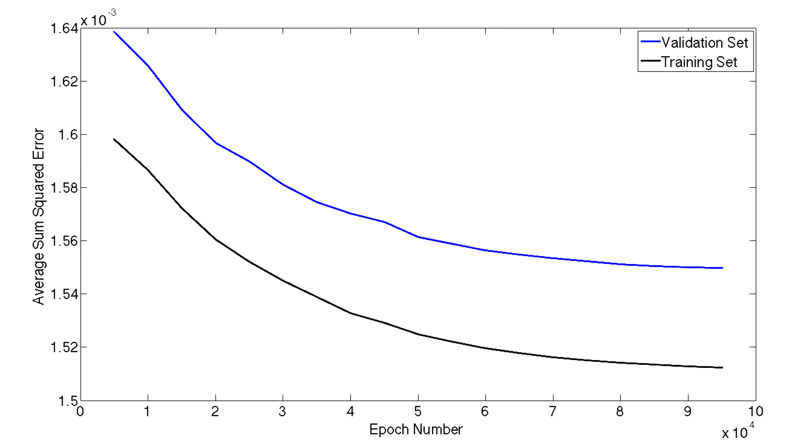
Figure 4
In an attempt to improve our results we switched from a regression problem to a classification problem and tried to model the posterior probability that there will be rain given our input variables. We did this by classifying any example where there was more than 0.1 inches of precipitation as a rain event with output value 1. We then re-ran our 10-fold cross validation on this new data set. Unfortunately, our results mirrored our previous attempt with the network learning to simply classify every example as a non-precipitation event. Figures 5 and 6 below provide our results from this case. Again we can see a very low number of misclassifications, in the 200-300 range out of a test set of 4383 examples. However, all the errors come from classifying a day when it actually precipitated incorrectly. So while our error rate is very low, it provides no beneficial information. Figure 6 shows the training of a neural network with 2 hidden layers and 20 nodes in the hidden layer.
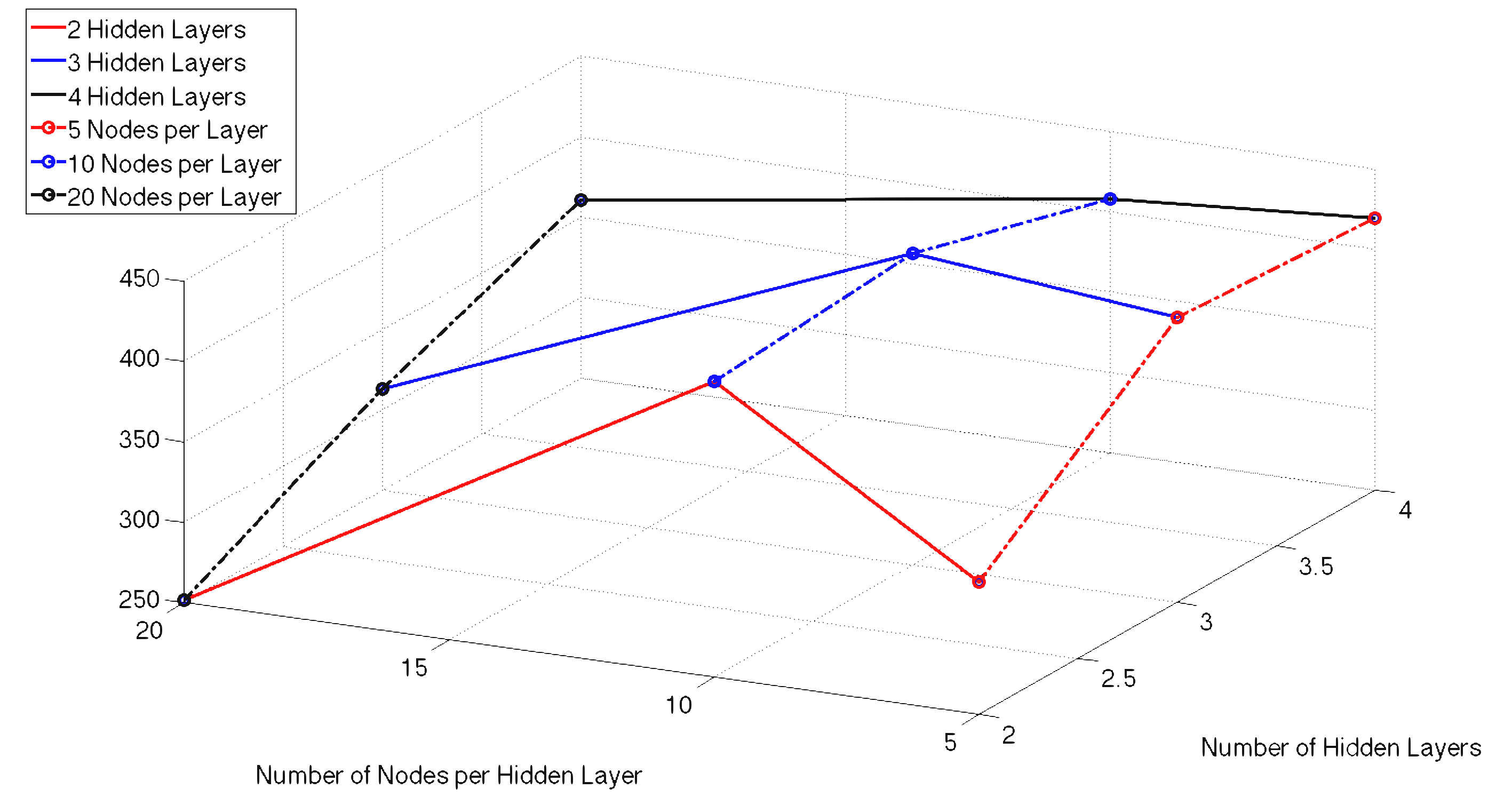
Figure 5
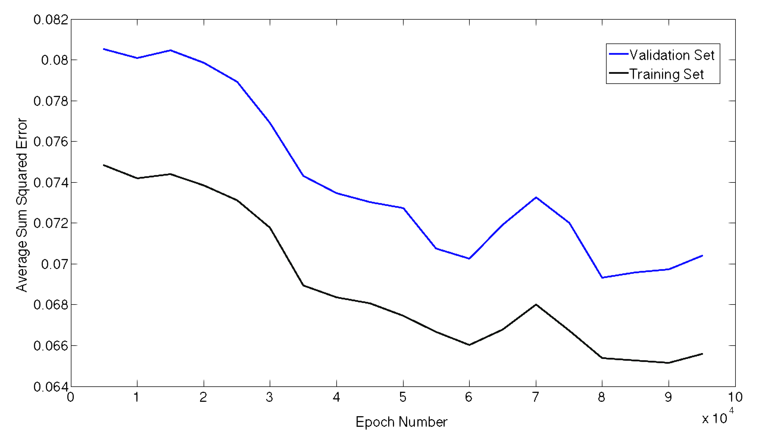
Figure 6
In an effort to improve performance we relaxed our prediction timeframe from 24 hours in the future to 6 hours in the future. Creating a random forest of decision trees using this new data proved more promising than before. Considering a subset of 100,000 possible splits at each node and an average of the posterior voting scheme for 20 trees, our decision tree had an error rate of 0.0488 on the test set. The error rate on precipitation events in the test set was considerably higher at 0.5633. This is a considerable improvement over our 100% error on the precipitation events when forecasting 24 hours in the future. Training a naive Bayes classifier on this 6 hour prediction data led to 100% misclassification of precipitation events on both the training set and test set, which is exactly what happened when trained for a 24 hour prediction. We are still working on training our neural networks on this new data set, and putting additional weights on examples where there was precipitation to normalize the skew of very few precipitation samples compared with many non-precipitation samples.
Plans
Because we have all of our data formatted and several algorithms fully coded, including our primary algorithm and two comparative ones, we are now in the process of producing better results. One of our problems stems from training our algorithms on data with significantly more samples without precipitation than with. Thus when we ran the algorithm on data we had reserved for test data, they classified everything or almost everything as 'no precipitation.' We are currently addressing this problem by weighting the error of precipitation training samples significantly higher than that of non-precipitation training samples in the optimization process. In the scope of our algorithm, we are also working to find the optimal number of hidden layers and nodes in the neural network to produce the best possible results. Implementing a radial basis function neural network is also something which we will try to do, as Santhanam and Subhajini found it to be more successful than a back propagation neural network in predicting precipitation (Santhanam).
In more general terms, we are starting smaller and trying to work up to a forecast of 24-hours. Right now we have stepped back and are testing and refining our algorithms for a 6-hour prediction with some success. After we have achieved adequate and consistent results on that time-frame, we will increase. As many of our sources, as well as numerical modeling and meteorology as a field suggest, precipitation forecasting is a difficult venture, even 24-hours in advance. We will also look into creating a form of a cascade predictor, where we first decide if there is going to be precipitation through classification and if so, proceed to predict the amount of precipitation through regression.
References
Bishop, Christopher M. "Neural networks for pattern recognition." (1995): 5.
French, Mark N., Witold F. Krajewski, and Robert R. Cuykendall. "Rainfall forecasting in space and time using a neural network." Journal of hydrology137.1 (1992): 1-31.
Ghosh, Soumadip, et al. "Weather data mining using artificial neural network." Recent Advances in Intelligent Computational Systems (RAICS), 2011 IEEE. IEEE, 2011.
Hall, Tony, Harold E. Brooks, and Charles A. Doswell III. "Precipitation forecasting using a neural network." Weather and forecasting 14.3 (1999): 338-345.
HPC Verification vs. the models Threat Score. National Oceanic and Atmospheric Administration Hydrometeorological Prediction Center, 2012. Web. 20 Jan. 2013. http://www.hpc.ncep.noaa.gov/images/hpcvrf/HPC6ts25.gif.
Hsieh, William W. "Machine learning methods in the environmental sciences." Cambridge Univ. Pr., Cambridge (2009).
Kuligowski, Robert J., and Ana P. Barros. "Experiments in short-term precipitation forecasting using artificial neural networks." Monthly weather review 126.2 (1998): 470-482.
Kuligowski, Robert J., and Ana P. Barros. "Localized precipitation forecasts from a numerical weather prediction model using artificial neural networks." Weather and Forecasting 13.4 (1998): 1194-1204.
Luk, K. C., J. E. Ball, and A. Sharma. "A study of optimal model lag and spatial inputs to artificial neural network for rainfall forecasting." Journal of Hydrology 227.1 (2000): 56-65.
Manzato, Agostino. "Sounding-derived indices for neural network based short-term thunderstorm and rainfall forecasts." Atmospheric research 83.2 (2007): 349-365.
McCann, Donald W. "A neural network short-term forecast of significant thunderstorms." Weather and Forecasting;(United States) 7.3 (1992).
Ming Leung, K. "Backpropagation in Multilayer Perceptrons." Polytechnic University. 3 Mar 2008. Lecture.
PSD Gridded Climate Data Sets: All. National Oceanic and Atmospheric Administration Earth System Research Laboratory, 2012. Web. 20 Jan. 2013. http://www.esrl.noaa.gov/psd/data/gridded/.
Santhanam, Tiruvenkadam, and A. C. Subhajini. "An Efficient Weather Forecasting System using Radial Basis Function Neural Network." Journal of Computer Science 7.
Silverman, David, and John A. Dracup. "Artificial neural networks and long-range precipitation prediction in California." Journal of applied meteorology 39.1 (2000): 57-66.
Veisi, H. and M. Jamzad, 2009. sc. Int. J. Sign. Process., 5: 82-92. "A complexity-based approach in image compression using neural networks." http://www.akademik.unsri.ac.id/download/journal/files/waset/v5-2-11-5.pdf.
Zhang, Guoqiang Peter. "Neural networks for classification: a survey." Systems, Man, and Cybernetics, Part C: Applications and Reviews, IEEE Transactions on 30.4 (2000): 451-462.