Flocking behavior of US equities
Ira Ray Jenkins and Tim Pierson
Dartmouth College Department of Computer Science
{jenkins, tjp}@cs.dartmouth.edu
Abstract
We've been working diligently on this project over the course of the term. Our first step was to produce a set of features that are analogous to flocks of real biological animals. We had to make a number of design decisions in developing our features, but at this point we're working with a set of 24 features. Since we are attempting to predict changes in equity prices over time, we also needed to decide how long into the future to look ahead to get the future equity price. Currently we're evaluating 1, 5, 10, and 20 minutes into the future. Our next step was to use Matlab's Neural Network Toolbox to review the data and begin making predictions. After an initial false alarm, we realized that our models were being swamped by the overwhelming number of cases where the price did not change significantly. As a result, we have switched gears and are developing a two-stage model. The first stage will simply predict if the stock will move over a period of time, but not which direction. The second stage model will train on cases where there was a significant price movement and will make predictions on the direction (e.g., up or down) the price will change. In essence the first stage is providing a filter for the second stage. In combination we hope these two stages will produce accurate predictions.
Developing the feature set
Separate companies into flocks according to industry sectors
Our idea was to model industry sectors as flocks of animals and individual companies within the sector as individual animals within a flock (e.g., 3M is in the Industrials "flock"). We had data on stocks in the Standard and Poor's 500 Index (S&P 500) and we used the industry classifications that S&P uses to categorize companies into groups. This gives us 10 flocks:
- Energy
- Materials
- Utilities
- Consumer Staples
- Industrials
- Financials
- Information Technology
- Telecommunications
- Health Care
- Consumer Discretionary
Focus on a particular flock — Industrials
We have data on the open price, high price, low price, close price, and volume in one-minute increments for the 500 stocks in the S&P500 for two years. This gives us over 2.3 billion features we could develop (500 stocks * 390 minutes/trading day * 252 trading days/year * 2 years * 24 features). To reduce this size we decided not to try to model all flocks at one time, but instead chose to initially focus on one sector.
We decided to initially focus on the Industrials sector for a number of reasons. First, our suspicion is that because the Industrials sector is less volatile than other sectors such as Technology or Energy, that it might be easier to make accurate predictions. This assumption, however, could end up being dead wrong.
Another reason to choose Industrials is because we had data for the entire period for 63 individual stocks. In some sectors such as Technology, companies join the S&P 500 Index and leave the S&P 500 Index more frequently (e.g., Facebook joins the Index, while last year's darling leaves the Index). The relatively large number of companies in the Industrials sector that stayed in the index for the entire period should help mitigate any unusual behavior of any particular company. Future work could consider the impact of companies coming and going. Here we try to purposely minimize it.
Build a model for each company? Not for now
Now that we have elected to focus on Industrials, one possible course of action would be to build a model for each company within the flock. While this approach might make a lot of sense, for example General Electric's stock probably does not behave exactly like ADT Corporation's stock, we have chosen not to take this approach for now. Time permitting we might experiment with this idea, but for now our approach will be to build one model for all members of the Industrials flock and make predictions for each company based on that single model. We hope that the less volatile nature of this sector will help a flock-wide model perform well. This assumption that a single model of the sector can perform well, like the assumptions above about the nature of the sector may prove to be incorrect.
Developing features based on biological flocks
Biologists have identified a number of features that model the dynamics of animal behavior within flocks. See Figure 1 for examples of emergent behavior.
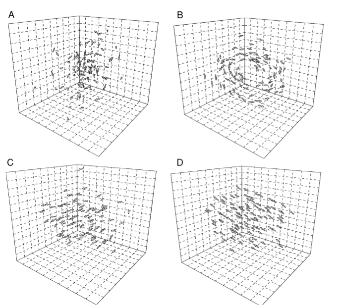
Figure 1.
Factors such as group polarity (e.g., the degree of alignment of individuals) and group velocity (e.g., how fast the group is moving) which are derived from characteristics of each individual animal can lead to the emergence of different behavior for the flock as a whole. Figure A show a "swarm" of animals milling about with low polarity and low velocity. Figure B shows a "torus", a flock with low polarity and high velocity. Figure C shows a "dynamic group", with high polarization and high velocity. Figure D shows a "highly parallel group" with high polarization and low velocity. From Couzin and Krause, 2003 [3].Inspired by the biologist's work, we have developed 24 features that have some analog to natural flocks. Some of the common features that biologists use in their models are:
- Position of an individual. Biologists use 3 dimensions for birds and fish, 2 dimensions for earth bound animals like wildebeest. We model stock position as 1-dimensional — the percentage change in price from the previous night's close. In our case, some stocks will be up, some will be down. We use percent change, as opposed to absolute change in dollars because stocks have varying prices. For example, a $700 stock that moves 1% will move $7. However, that same $7 movement would be a 70% move for a $10 stock. By using the percent change we normalize this concept and make it easier for the model to deal with.
- Velocity of an individual. Biologists use the animal's actual speed. We are using the number of shares traded (see below for difficulties in this) to represent velocity.
- Rank of an individual. In some biological groups individuals have different social rank and can influence the group's behavior more than others. Think of a lion pride, where one lion is the "king" and can influence the actions of other lions more than a lion of lower status can influence other lions. We model this effect by including the market capitalization of the individual stocks.
- Direction an individual is facing. Biologists can use a compass heading based on where the animal's nose is pointing. We are using the slope of a linear regression of the recent stock prices. In our case, some stocks will be pointed up (e.g., prices have been increasing as indicated by a positive regression slope) or pointed down (e.g., prices have been decreasing as indicated by a negative regression slope), or pointed straight ahead (e.g., indicated by a close to zero regression slope).
- Center of the flock. Center point of all animals in the flock. We model this as the average change in price from the previous night's closing price of all individuals in the flock.
- Velocity of the flock. How fast the center of the flock is moving over time. We model this as the average velocity of individuals in the flock (see below for difficulties in modeling this).
- Direction of the flock. This is the change in coordinates of the center of the flock over time. We model this as the average direction all individuals are facing.
- Polarity of the flock. This is how aligned individuals are in the flock. In some instances individuals are milling about, facing in different directions (see Swarm in Figure 1 above). In those cases, the group's polarity is low. In some cases the group is moving purposefully in a specific direction. In this case, the group has high polarity. We are modeling polarity as the standard deviation of the direction all individuals are facing (e.g., are they all going up, or all going down, or relatively flat). A low standard deviation suggests a high polarity.
- Flock density. This is how tightly packed the flock is. We model this as the standard deviation of the position of all individuals. As described above, the position of each individual is the percentage change in price from the previous night's closing price. A low standard deviation of all individuals' positions suggests a high density.
- Time of day. In the real world, animals behave differently at different times of day. For example, some animals sleep during the day and are active at night (like grad students?). Others are reversed. We model difference in behavior at different times of the day by providing the model the number of minutes since the market opened for each feature.
Below is a brief summary of our model features, grouped by stocks and sectors, and their biological analog.
| Biological Feature | Market Feature |
|---|---|
| Individual Stocks | |
| Position | Percent change in price from previous night's close |
| Velocity | Z Score of number of shares traded per minute for the current minute and previous four minutes |
| Rank | Market capitalization |
| Direction | Linear regression slope of recent prices for 1, 5, 10, and 20 minutes |
| Sector "Flocks" | |
| Center | Average change in price from previous close of all individuals |
| Velocity | Average of velocity of all individuals for current minute, plus previous four minutes |
| Direction | Average of direction all individuals have been facing for 1, 5, 10, and 20 minutes |
| Polarization | Standard deviation of direction of all individuals for 1, 5, 10, and 20 minutes |
| Density | Standard deviation of change in price from previous close of all individuals |
| Time | Minutes since the market opened |
Difficulty modeling some features
Some features were difficult to model. For instance, we wanted to model the velocity of particular individual as the number of shares traded recently. But, two issues confounded that. First, volume is very inconsistent. For example, in Figure 2 below we see a big change in the volume of shares traded each minute. This happens very commonly in the market.
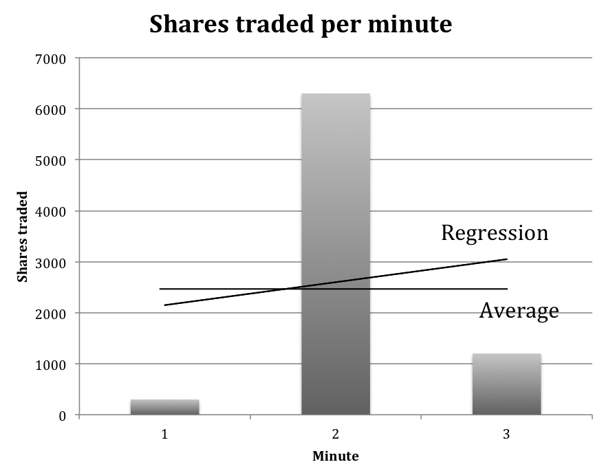
Figure 2.
Variance in shares traded. This figure shows how the number of shares traded per minute can vary substantially over a short period of time. Here we show the number of shares traded for a particular company over a three-minute period. The question then is how to model this. One approach might be to take the average number of shares traded. This approach, however, may not be a good indication of the velocity. Another approach might be to do a linear regression over a small time period and use the slope. Again, this approach might not serve a model well.Our approach is to first calculate a Z score for each minute of trading. This is calculated by first determining the average number of shares traded per minute of each trading day (this varies considerably during the day, where right after the market open and right before the market close average share volume is typically much higher than during the middle of the day) and the standard deviation of the number of shares at each minute. Then for each sample, we take the current shares trades and subtract the average shares traded for that minute. We divide this by the standard deviation of the number of shares traded.
Z = (current volume - average volume)⁄standard deviation of volume
In this way we normalize a score for all stocks, whether they trade relatively high volumes or whether they trade relatively low volumes.
Once the Z score is calculated, we provide the model with the current Z score and the previous four minutes' Z scores (a total of five minutes). In this way we let the model determine what is most important, rather than providing a summarized metric such as the average score or slope of a linear regression of volume traded over five minutes.
Developing target values
We are trying to predict the movement of stock prices based on what the flock is doing at any particular point in time. One natural question that arises then is how far into the future should we predict. We decided to develop targets that are the percentage change in price (so we can more easily handle difference in the magnitude of stock prices, $700 vs. $10) for 1, 5, 10 and 20 minutes into the future. The Efficient Market Hypothesis tells us the price in the near future should be the price it is currently, but we see clearly that prices will drift more over longer periods of time. Our presumption is that it will be easier to accurately predict the price 1 minute into the future than it will be to predict 20 minutes into the future. Nevertheless, we developed targets for each of these time periods to investigate temporal effects.
Test results looked promising at first, then reality set in
Because our data is a time series, we first decided to investigate Matlab's time series Neural Network tools. We initially selected the Nonlinear Autoregressive with External Input (NARX) tool and ran it with our data. The results were spectacular (see Figure 3 below).
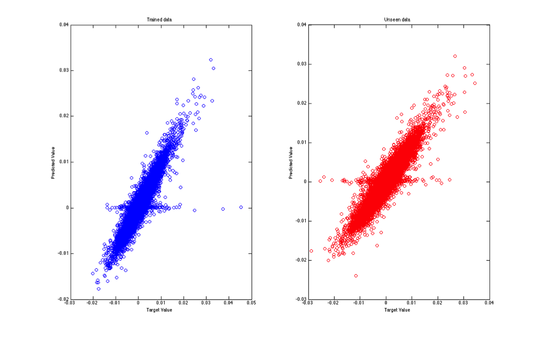
Figure 3.
NARX results. This figure shows the performance of the NARX neural network on roughly 100,000 samples while trying to predict price changes 20 minutes into the future. The x-axis shows the actual target value (e.g., the price 20 minutes in the future). The y-axis shows the model's predictions. The left figure shows performance vs. training data. The right figure shows performance vs. testing data. If the model were perfectly accurate the points would align at a 45-degree angle. This shows performance very close to that.As we dug deeper into how NARX networks work, we realized we had a problem. In the NARX topology, target values are fed back into the model, making it a recurrent model. In our case, however, y(t) is the value of the price change some time period in the future. Here the time period was 20 minutes. See Figure 4.
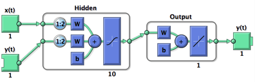
Figure 4.
NARX Neural Network. Diagram of a NARX neural network. Notice that the true values of the targets, y(t), are feed into the model. In our case this would be the price change 20 minutes into the future lagged by one minute, giving the model the chance to make a prediction of the price change 20 minutes into the future using the price change 19 minutes into the future as an input. Graphic from Matlab documentationA closed loop version of the NARX network would use the predicted value (e.g., model output, not the true value) of the previous minute as input into the next prediction and this may be an area to examine in the next phases. For now, however, we decided to use a non-recurrent version of the Matlab Neural Network Toolbox to make sure we've eliminated this potential complication.
When we ran the model again using the Matlab Fitting Tool to perform a regression against the change in price 20 minutes into the future, we saw a remarkable decrease in performance. Reality had set in. Our network wasn't performing as well as we'd hoped. See Figure 5.
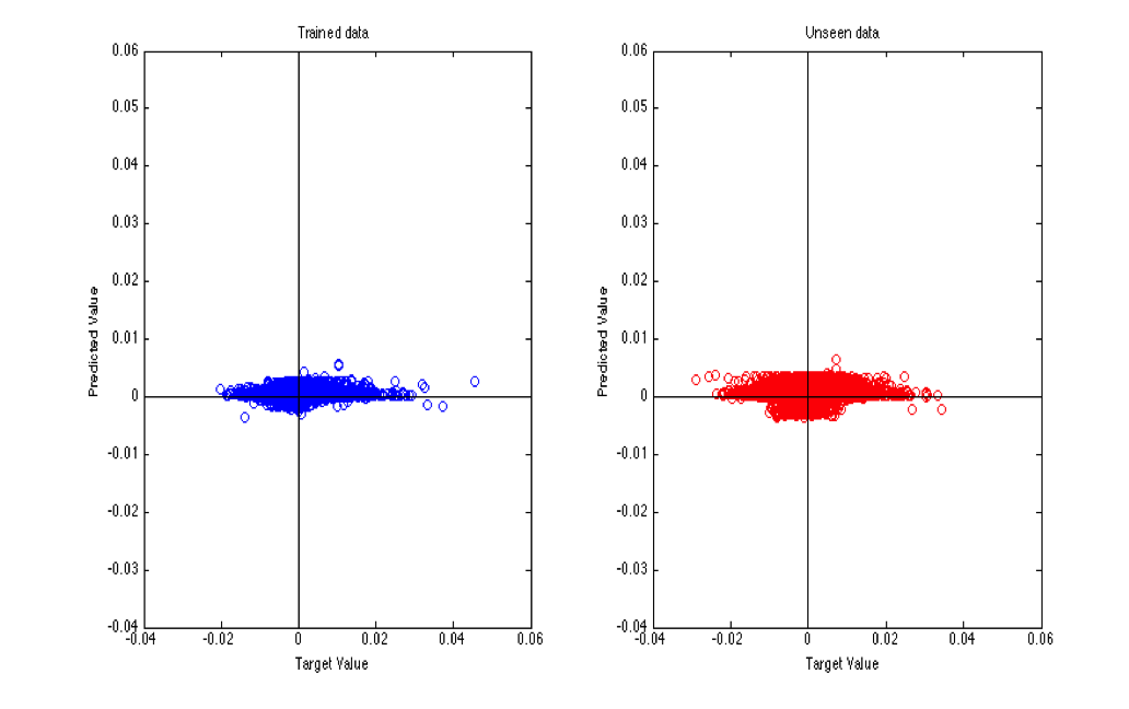
Figure 5.
Matlab Neural Network Fitting Tool performance. This figure shows the performance of the Matlab Neural Network Fitting Tool on roughly 100,000 samples while trying to predict price changes 20 minutes into the future. As before, the x-axis shows the actual target value and the y-axis shows the model's predictions. The left graph shows the performance against training data. The right graph shows the performance against test data. In both case the predicted movements are close to zero.When we reviewed the target data more closely, we saw the culprit. The vast majority of inputs, even when looking 20 minutes into the future showed near zero movement. See Figure 6.
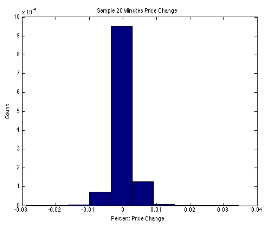
Figure 6.
Histogram of price changes 20 minutes in the future. This figure shows a histogram of the percentage price change of a sample of nearly 100,000 target values. The vast majority of those inputs have nearly no price over the 20-minute period. While not shown, the number of samples showing a significant movement (say 0.5%) is even smaller for shorter prediction time periods (e.g., 1, 5 or 10 minutes).The fact that relatively large price changes are uncommon, even when looking 20 minutes into the future means our model was able to do a reasonably good job overall if it predicted nearly no movement. This stands to reason. If 99% of the time there is no movement, then simply predicting no movement means the model will be accurate 99% of the time. That, however, is not useful for our purposes. We are specifically looking for cases where the stock will reliably have a significant price change
New approach — model this as a two-stage problem
After speaking with Dr. Torresani, we came up with a new plan to overcome these obstacles. We are modeling this as a two-stage problem. The first stage is to train a neural network to detect if the stock will have a reasonably significant price change over the next few minutes. This stage simply outputs one if the stock is predicted to move, it could move either up or down, otherwise it outputs zero. The second stage predicts which direction the stock will move, up or down, only if the first stage predicts a significant price change. In a sense the first stage is providing a filter for the second stage.
First stage — predict if there will be a significant price change
The first stage's task is to predict when a stock will make a significant price change. We are now modeling this as a classification problem, whereas previously we'd modeled it as a regression problem. That is to say, previously we were predicting the percentage change in price as a real value, now we are predicting a class of type one if the price will make a significant move and a class of type zero otherwise.
Three questions naturally come to mind given this approach:
- What constitutes a significant price change? We've decided to use 0.5% as a threshold denoting a significant price change. This choice is not entirely arbitrary, but is also not entirely rigorously selected. We could use a smaller move, but we are concerned that it will result in more noise for the model to contend with. With a smaller value for a significant price change, if the stock were moving randomly as in the "Swarm" configuration in Figure 1 above, then sometimes the stock would randomly cross the this threshold, even though it was moving as a random walk. Using a higher threshold helps to prevent that. Using a value that is too high, however, would reduce the number of samples that actually make the move. For instance, looking one minute into the future, approximately 0.3% of samples have a price change at our level. Increasing the required move would result in fewer samples displaying a significant move and give the model less data to use to discriminate between movers and non-movers.
- How far into the future should we try to predict? As noted above, we have developed target data for the percentage change in price for 1, 5, 10, and 20 minutes into the future. It is currently unclear how far we should try to predict. Our suspicion is that making predictions over a shorter time period will be more accurate overall, but will likely result in smaller predicted movements because the stock price will have had less time to vary. We are currently running models to evaluate how far to look into the future. See Figure 7 below.
- How many neurons should be in the hidden layer? Another issue is network configuration. A smaller network, with a smaller number of neurons in the hidden layer, will likely be more resistant to over fitting, but might not have enough computational power to discern subtle signals of an impending price change. To understand this, we are currently running models to evaluate how many neurons to use. See Figure 7 below.
To better understand issues 2 and 3 above, we are using 5-fold cross validation against our training data. It should be noted that a single run takes about 18 hours. Because we have 7 million rows of inputs and targets, and we would like to try multiple time periods and network configurations (and we need to use our computers for other class work), we are doing random sampling of our data to test the various setting. The following is pseudo code for our current effort to choose our configuration optimally:
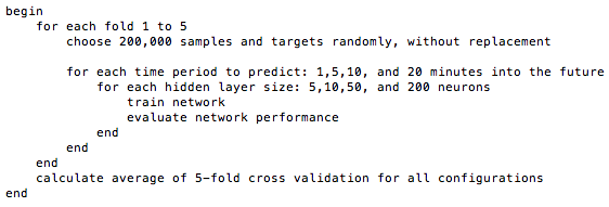
This work is currently ongoing and this algorithm takes a long time to complete. We've run into issues where the VPN timed out, killing some runs we attempted to make from home. We've also had to kill some runs from inside Sudikoff because we needed our computers for other classes. We did, however, get one run to complete and results are shown below in Figure 7.
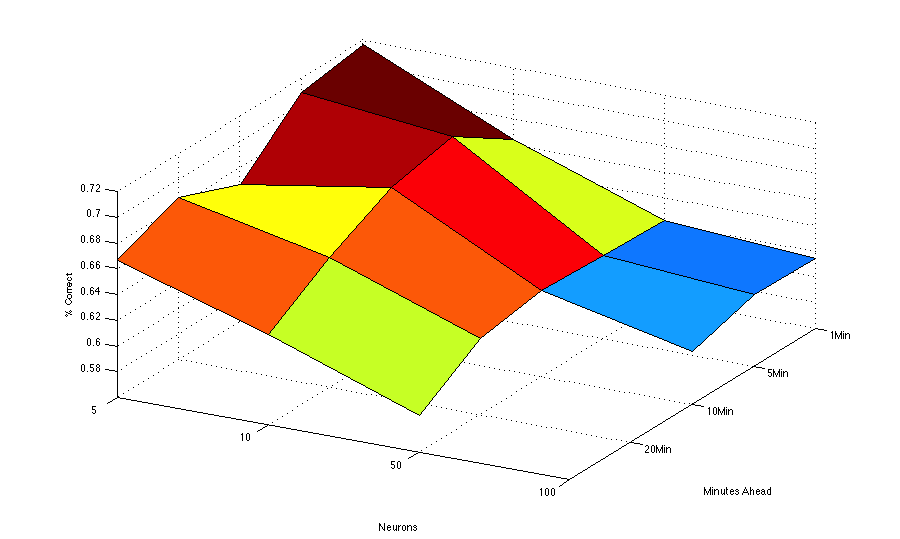
Figure 7.
Surface plot of various configuration options. This figure shows the number of neurons in the hidden layer on the x-axis and the number of minutes ahead to predict price changes on the y-axis. The percentage of correct model outputs where a class of one is predicted is show on the z-axis.There are two important points to make about this surface plot. First, this was done with one run with 100,000 samples, not a 5-fold cross-validation, so it may show some peculiarities of the particular samples that were selected. It suggests, however, that making predictions over a shorter time period is generally easier than making predictions further into the future, but curiously, it suggests that a small number of neurons is all that is required to make the best predictions. This would suggest that more neurons are causing over fitting. Other runs we're currently making are suggesting more neurons make better predictions. We will have a better sense of this once our 5-fold cross-validation completes.
The second major point about this surface plot involves the values on the z-axis. In a real-world stock-trading situation, we would be most concerned about cases where the model predicted a significant price movement, but none occurred. We might use the model's output as a signal to buy shares in a company. If it failed to move, we would not make a profit (although we would not loose much money). As a result, we plot on the z-axis the percentage of time the model predicted a significant price movement and a significant price movement actually occurred. The model outputs a value in the range [0,1]. Currently if the value is greater than 0.5 we declare the output to predict a significant price movement. This value, however, could be adjusted so that the model will would have to be more confident before we declare a likely significant price movement. We could, for instance, set this threshold to 0.75. In this way the model would predict a fewer number of significant price moves, but it would be more confident when it does.
In the interest of completeness, there is another type of error the model could make that we are less concerned about. The model could predict that the stock would not experience a significant movement over the time period, and a significant movement could occur. In a real-world stock-trading situation, we could view these cases as an opportunity cost. We missed the opportunity to take part in a price movement, but we are less concerned because we would not have put capital at risk. Ideally, however, our model would catch most of these instances and alert us to the possibility of a significant price movement.
In the end, there may be a trade-off to be made between making a smaller number of more accurate predictions or a larger number of less accurate predictions. Either case could be profitable. For example, making a stock trade one time per week and getting it right 100% of the time with a profit of 0.5% at each trade would be less profitable over time than making one stock trade per day and getting it right 80% of the time on average. Time permitting, we will investigate this, but it is likely an area for future work.
Second stage — predict the direction (e.g. up or down) of a significant move
We have not yet begun working on the second stage of our model, but it will attempt to determine the direction (e.g., price goes up or price goes down) when a significant move is predicted by the first stage. We expect to model this as a classification problem with two classes: price will go up, or price will go down. In order to train the model, we will identify all training examples where a significant movement actually occurred and we will label those instances as either will go up or will go down. We will then test various network sizes to try to determine the optimal configuration. Our plan will be to use the optimal number of minutes to look ahead for a price change that was determined in our current work on the first phase. Future work might reverse this and look at optimizing the second, direction prediction stage first, then use that look ahead period for the first stage. We would then be able to decide on which approach yields the best results.
Summary
We have met the milestone goals set in our project proposal. We have collected our data, derived our feature set, and completed a few runs using our initial neural network model, as well as the new multi-stage network. There remains potential for our hypothesis to be proven correct, and we believe we are on-track to complete our project successfully.
Next steps
For the rest of term, our plan is to refine our work on the first stage of the two-stage model. After that is complete we should have determined the optimal time period to make predictions, and the configuration of the first stage neural network. We will then move on to stage two and complete it as described above. As time permits we may:
- Evaluate other industry sectors, perhaps Technology as a contrast to Industrials
- Use a closed loop recurrent network configuration
- Try building a model for each company within the flock and see if a company-specific model outperforms a flock-wide model
- Change the confidence required to predict a movement
- Build the two models by first optimizing the second stage model that predicts direction on time period and using that as the time period for the first stage model to predict if there will be a price movement.
References
- William Bialek, Andrea Cavagna, Irene Giardina, Thierry Mora, Edmondo Silvestri, Massimiliano Viale, and Aleksandra M. Walczak. Statistical mechanics for natural flocks of birds. Proceedings of the National Academy of Sciences, 109(13):4786–4791, 2012.
- S. Camazine, J.L. Deneubourg, N.R. Franks, J. Sneyd, G. Theraula, and E. Bonabeau. Self–organization in biological systems. Princeton University Press, 2003.
- Iain D Couzin and Jens Krause. Self–organization and collective behavior in vertebrates. Volume 32 of Advances in the Study of Behavior, pages 1–75. Academic Press, 2003.
- Burton G. Malkiel. A Random Walk Down WallStreet: The Time–Tested Strategy For Successful Investing. Norton, New York, NY, USA, 2003.
- Burton G. Malkiel and Eugene F. Fama. Efficient capital markets: A review of theory and empirical work. The Journal of Finance, 25(2):383–417, 1970.
- Craig W. Reynolds. Flocks, herds and schools: A distributed behavioral model. In Proceedings of the 14th annual conference on Computer graphics and interactive techniques, SIGGRAPH '87, pages 25–34, New York, NY, USA, 1987. ACM.
- J.D. Schwager and J. Greenblatt. Market Sense and Nonsense: How the Markets Really Work (and How They Don't). Wiley, 2012.
- Matlab. Neural Network Toolbox. MathWorks. February, 2013. http://www.mathworks.com/products/neural-network/