CS74 Project Milestone

Introduction:

Deep Networks are a very up-and-coming machine learning technology. Just yesterday, Android's NN voice recognition made the homepage of Wired, and Deep Learning research has made it into the NY Times and the New Yorker. A Deep Network, in the simplest sense, is a multi-layered Neural Network. These have shown to be effective, but unfortunately very time consuming to train. Our goal is to use the power of parallel programming to speed up the training of a neural net. To do this, we will have a sequentially trained neural net that we'll use as a control, and compare this to the performance of a parallelized training algorithm.

Dataset:

To test our networks, we chose a data set with a large number of attributes, and also a large number of training instances. This gives us room to demonstrate the power of the parallel approach, especially since visual and audio processing (with unweildy numbers of inputs and instances) are the most popular way to use these nets. Our data set was a little less glamourous: A forest cover type classification problem, given 54 attributes of the area in consideration. In short, we had 54 inputs and 7 outputs. We normalized the input so that they fell into the 0-1 range, and we set up the output to be binary classifiers, 0 or 1 for each of the seven possible cover types.

Results:

Sequentially Trained Net

We have completed, optimized, and tested the sequentially trained net. Before we could run tests, we had to first settle on a few hyperparameters. Specifically, the number of hidden nodes and the learning rate. We found appropriate values through simple testing and plotting, and settled on 50 hidden nodes and a learning rate of 0.3. We used Stochastic Gradient Descent (SGD) with Back Propogation to train the net.

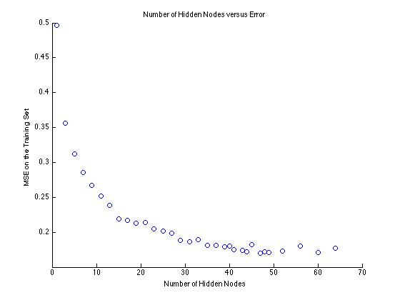
Figure 1. Choosing the number of Hidden Nodes. Too many nodes leads to overfitting, too few gives underfitting.

Next we looked at how the training was proceeding. Here we look at the error over number of iterations, or epochs, of gradient descent. As we expect, error decreases. We are using a stochastic gradient descent, though, so there is a degree of randomness, visible here as spikes. This can be very beneficially for getting out of local minima, and we hypothesize that that's what happened with this spike and drop near the end of the iterations.

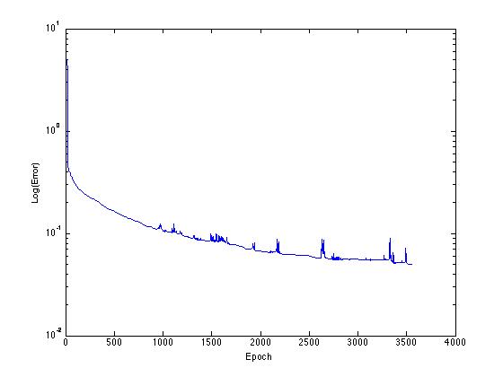
Figure 2. Training of the sequential model with Stochastic Gradient Descent.

So running many epochs is clearly beneficial to this network, as is increasing the size of the training set. But what is that costing us in time? Well, unfortunately, it's expensive. This plot here, of number of training examples versus time, shows a clear linear trend, and our trials also showed that more examples take more epochs, which compounds this issue. In short, this is not feasible for scaling up.

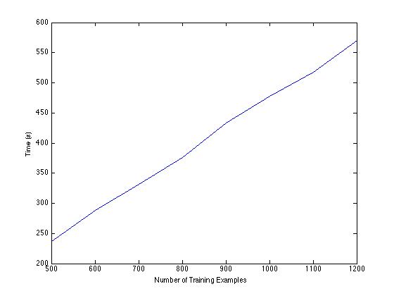
Figure 3. Correlation of the size of the training set and training time.

Parallelization to the Rescue!

This is the parallel model we'll be using, inspired by work done Dean et al. [1] on what they call Downpour SGD. It takes the inherently sequential training algorithm, SGD, and tries to split up the work. You have a server of parameters (the weights that you are trying to optimize), and a group of clients that are all individually running SGD on data shards. Periodically, the clients tell the server what changes they've made to the parameters. The server takes the updates, and updates its master copy of the parameters. The clients also periodically request the parameters from the server, and the servers sends that client the master copy. The clients all run asynchnously, so there doesn't need to be any communication between them. Only the parameters and updates need to be broadcasted, and only between the server and clients. Notice that the clients are not necessarily always running with the most recent set of parameters. They might run SGD and find updates on an outdated copy. This introduces another degree of randomness, that the original researchers actually found to be very benefical for keeping the model out of local minima.

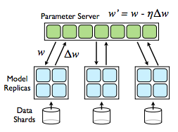
Figure 4. Depiction of the parallel training model, from [1].

Expected Speed Up

A standard measure of the degree of parallelism one can achieve with an algorithm is speedup. Speedup is the ratio between the amount of time it takes to complete a task on one processor and the amount of time it takes to complete that task with p processors. An ideal speedup is linear speedup, where the value is p. In this case, assuming a sufficiently large input such that each processor has something to do, the more processors you have the faster the computation is, with no upper ceiling.

SGD iterates over all the examples in the training set of size s, calculates the error for each, and then updates the parameters. In the parallel implementation with p processors, however, it runs a standard SGD over a training set of s/p. As discussed previously, this isn't totally equivalent to SGD, which depends on the parameters of the previous iterations (an inherently sequential operation). However, this parallelized SGD still converges on a minimum, and we expect it to do so at a rate similar to the sequential case, aside from a little more noise. This therefore gives us linear speedup, and indicates that it is a prime candidate for parallelization.

Implementation

To actually implement this algorithm, we investigated several parallel programming paradigms: CILK, CUDA C, and MPI.

Cilk is a programming language, very similar to ANSI C, with several keywords that fork the program into parallel processes into seperate threads and later sync them back together. Although this would be simple to implement, Cilk is designed for Symmetric Multiprocessors, which all have access to a single main memory. With the ultimate goal of making the parallel SGD scalable, this would be problematic, because the whole data set would NOT neccessarily fit on a single main memory.

Another common approach, widely researched, is the use of a GPU. A GPU is the graphics card on a computer, and it has an architecture consisting of a large number of multiprocessors. Additionally, nVidia has a language similar to C, called CUDA C, which can be used to program their GPU's. This gives us a highly parallel architecture to use. However, once again, scalability becomes a problem because GPU's have severe memory limitations (6 GB) and don't communicate between each other easily or well.

Lastly, we have MPI (Message Passing Interface), which is a communication protocol with an implementation as a library in C. MPI provides communication functionality between a set of processes, each which has been mapped to a node in a cluster. Since MPI revolves around broadcasting and recieving data like the algorithm we are using, and each process is mapped to a node with its own memory, MPI fits our problem intuitively and is open to massive scalability.

Pseudocode

Here is the specific pseudocode for the algorithm, implemented with MPI in mind. The main things to note is the fetching and pushing of parameters (lines 18 and 33). In between those two operations is a typical SGD, that closely resembles what we used earlier in the sequential case. We are particularly excited about how generalizable this algorithm is; it makes no distinction between regular Neural Nets and Deep Nets, or even the use of an ANN at all. We expect that this will be similarly effective for any algorithm that uses Stochastic Gradient Descent.

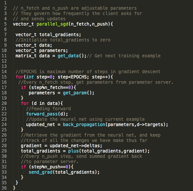
Figure 5. Our pseudocoded algorithm.

Milestone Evaluation

We are still on track with our project. We've changed the originally proposed data set to something of more managable size. Since our focus is on the algorithm we didn't want to have to spend time pre-processing a complex data set.

We expect to get the parallel training algorithm running very soon, and will start collecting final data. We were surprised at how long it takes even modestly sized training sets to run, so we need to make sure that we have plenty of time to collect all of the results.

Reference: