Samuel Nastase & Hsin-Hung Li
Machine Learning and Statistical Data Analysis
Dartmouth College
2013
The current project aims to investigate how bottom-up attentional signals are computed by the brain using a neurally-inspired model of visual saliency. When sudden changes occur in our visual environment, the brain rapidly processes this information in order to direct the eyes toward the salient target. These saccades bring the target into foveal vision, affording higher visual acuity. The overarching goal of our project is to use recently developed visual saliency model (Itti & Baldi, 2009; Itti & Koch, 2001) to predict voxel time series of subjects watching the movie Indiana Jones – Raiders of the Lost Ark. This method of model-based neural decoding using functional MRI (fMRI) has proven useful in explaining how the brain represents early visual and semantic information (Huth, Nishimoto, Vu, & Gallant, 2012; Mitchell et al., 2008; Nishimoto et al., 2011). By the milestone, we had intended to have a working replica of the visual saliency model, have preprocessed and hyperaligned the fMRI data (Haxby et al., 2011), and have coded the learning algorithm necessary to optimize model parameters.
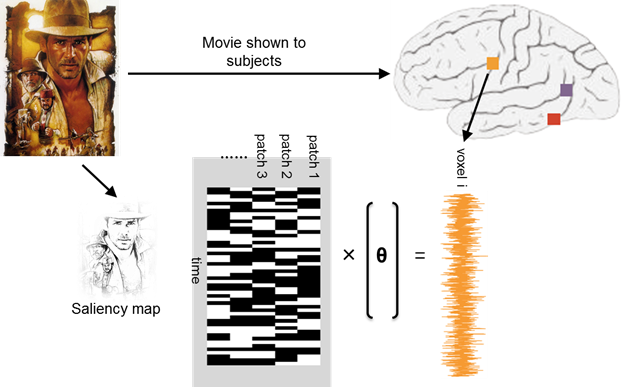
Figure 1: Schematic depicting voxelwise model estimation.
So far, we have successfully applied a stripped-down version of the saliency model to a single 14 min segment of the movie stimulus. The iLab Neuromorphic Vision C++ Toolkit (iNVT) was used to compute saliency maps for each from of the movie. Specifically, this model simulates functional properties of visual neurons in the retina, lateral geniculate nucleus (LGN), and several areas of early visual cortex, including primary visual cortex (V1) and visual area MT. For example, the model incorporates the center-surround opponency receptive field structure of LGN neurons. For each movie frame, the model decomposes the input image according to several feature maps. The channels we elected to use are center-surround intensity, center-surround color opponency, orientation contrast, center-surround motion energy, and center-surround flicker detectors. These filters operate over six spatial scales for each channel. A single saliency metric is then computed over all of these feature maps at each image patch, resulting in a single saliency map for each movie frame. These saliency metrics were computed at the native frame rate of the movie (30 Hz). These saliency maps were then temporally down-sampled in order to interface with the low temporal resolution of the fMRI data (2.5 s sampling rate). Saliency maps were then imported into MATLAB and concatenated in order provide a time series of saliency values at each image patch for the initial 14 min segment of the movie. These maps correspond to a 2,718 (time points) × 1,908 (image patches) matrix of saliency values. Coefficients of these saliency values at each image patch comprise the model parameters to be optimized.
Figure 2: Example movie frames and corresponding saliency maps.
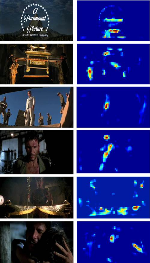
Figure 3: Accelerated saliency map movie. Saliency Movie
Furthermore, we fully preprocessed the fMRI data in order to prepare them for regression. Initially, only a single run corresponding to the initial 14 min movie segment was analyzed and all preprocessing was done in AFNI (Cox, 1996). Preprocessing consisted of first spatially registering all volumes of blood oxygenation level-dependent (BOLD) responses across all runs within a single subject to a single reference volume. Slice-timing alignment was performed to correct for small temporal disparities in slice acquisition within a single volume. BOLD time series were then despiked and bandpassed in order to account for any low frequency drift in the MR signal. Finally, head motion parameters derived from initial spatial registration were then regressed out of BOLD time series. Additional preprocessing steps, such as applying a 4 mm spatial smoothing kernel, may be implemented in the future in order to optimize model performance, although it is unclear a prior whether these steps will be beneficial. Furthermore, although we have successfully hyperaligned fMRI data across subjects, we have elected not to include this in the current analysis yet in favor of first validating our method in a single subject. These fully preprocessed BOLD data were then multiplied by a binary mask in order to negate any voxels not in the brain and were converted to a MATLAB-compatible format using pyMVPA. The resulting 2,718 (time points) × 71,773 (voxels) matrix of BOLD response values was imported into MATLAB. The vectors of 336 BOLD values for each voxel comprise the target values to which the model will be fitted.
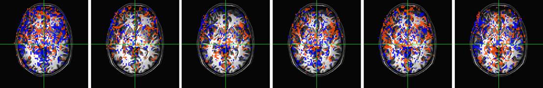
Figure 4: Neural activity corresponding to above movie time points.
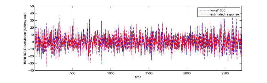
We are currently implementing support vector regression (SVR; Drucker, Burges, Kaufman, Smola, & Vapnik, 1997) to estimate the response of each voxel as a linear combination of the saliency values at each time point. At the moment, we are using the Smooth Support Vector Machine toolbox (Lee & Mangasarian, 2001) in MATLAB to kick-start this analysis, although we may yet abandon this toolbox. For each voxel, this procedure results in a set of model weights applicable to the corresponding saliency map values. These model weights reflect how strongly visual saliency information as quantified by the model captures voxel activity. As a baseline measure, we are also implementing a simple linear regression to the same end, although we expect that SVR will outperform linear regression once we have optimized SVR hyperparameters. Unfortunately, as of now we have only been able to apply these two regression techniques to a single voxel in a single participant. While the basic linear regression appears to successfully estimate voxel time courses, we have not yet been able to properly apply SVR—currently the SVR returns a single value for all model weights.
Figure 5: Estimated voxel time course based on linear regression compared to actual voxel time course.
In the coming weeks, we hope to expand our analysis on several fronts. Most importantly, we plan to debug the SVR procedure in order to accurately estimate voxel time courses. Once the SVR procedure is working properly, we will iteratively estimate time courses for all voxels in the brain. Then, we will implement a leave-two-out cross validation scheme in order to determine whether the learned model parameters generalize to novel segments of the movie stimulus. Predicted voxel time courses will be generated for a left-out segment of the movie and we will test whether these simulated activity patterns more closely resemble the actual brain data for the corresponding or the alternate left-out segment.
References
Drucker, H., Burges, C. J., Kaufman, L., Smola, A., & Vapnik, V. (1997). Support vector regression machines. Advances in Neural Information Processing Systems, 155-161.
Haxby, J. V., Guntupalli, J. S., Connolly, A. C., Halchenko, Y. O., Conroy, B. R., Gobbini, M. I., Ramadge, P. J. (2011). A common, high-dimensional model of the representational space in human ventral temporal cortex. Neuron, 72(2), 404-416.
Huth, A. G., Nishimoto, S., Vu, A. T., & Gallant, J. L. (2012). A Continuous Semantic Space Describes the Representation of Thousands of Object and Action Categories across the Human Brain. Neuron, 76(6), 1210-1224.
Itti, L., & Baldi, P. (2009). Bayesian surprise attracts human attention. Vision Research, 49(10), 1295-1306.
Itti, L., & Koch, C. (2001). Computational modeling of visual attention. Nature Reviews Neuroscience, 2(3), 194-203.
Lee, Y.-J., & Mangasarian, O. L. (2001). SSVM: A smooth support vector machine for classification. Computational Optimization and Applications, 20(1), 5-22.
Mitchell, T. M., Shinkareva, S. V., Carlson, A., Chang, K. M., Malave, V. L., Mason, R. A., & Just, M. A. (2008). Predicting human brain activity associated with the meanings of nouns. Science, 320(5880), 1191-1195.
Nishimoto, S., Vu, A. T., Naselaris, T., Benjamini, Y., Yu, B., & Gallant, J. L. (2011). Reconstructing visual experiences from brain activity evoked by natural movies. Current Biology, 21(19), 1641-1646.