**Matthew Ellison & Leah Ryu CS87 Final Project**
**by Leah Ryu (F003MC1) and Matthew Ellison (F004SPK)**
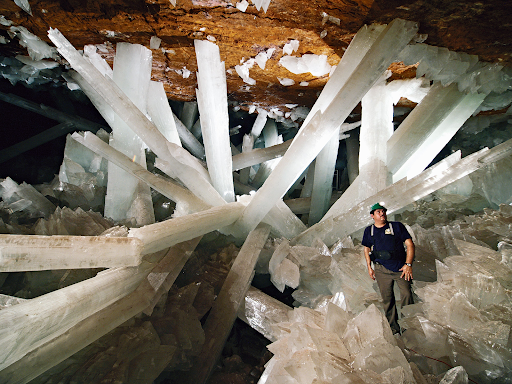
Motivational images
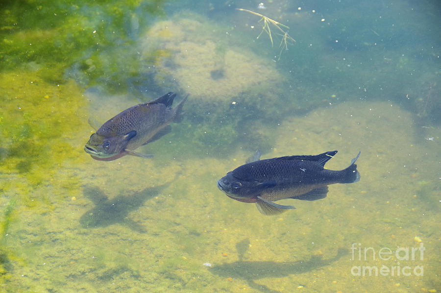
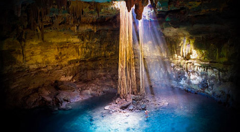
We were interested in building a night scene of a cave with crystals. We wanted to have a fish in the cave, which, to match the theme, would cast the shadow of it's inner spirit, a dragon.
Here are a number of motivational images:
Fish shadow https://pixels.com/featured/fish-casting-shadows-jeff-swan.html)
Light streaming into cave https://blog.investmentpropertiesmexico.com/lifestyle/4-must-visit-underwater-caves-in-mexicos-yucatan-peninsula
Theme
The connection to the theme (it’s what’s on the inside that counts) is illustrated by the relationship of the fish to the dragon shadow--it’s a common theme across several Asian mythologies that a koi can, through hard work, transcend and become a dragon. Additionally, we are hoping to evoke the mood of a hidden grotto within the earth, which more obliquely references the theme of interiority.
Features
Volumetric & Subsurface Scattering Path Tracing
Homogeneous Henyey-Greenstein medium
Code:`src/media/homogeneous_henyey-greenstein.cpp`; `include/medium.h`.
We first implemented a basic homogeneous volumetric path tracer using the Henyey-Greenstein phase function.
The Henyey-Greenstein phase function takes in three parameters:
g : average cosine g representing the balance of forward and back-scattering
sigma_t : total extincion coeffient which determines how frequently volumetric scatters occur
sigma_s : how much light scatters at each volumetric scattering event
By adjusting these three parameters we can simulate a variety of media.
Implementing this required a fair amount of additional plumbing, as I'm sure the grading reader knows. This included making the Li call take
current media as a parameter, and adjusting the json file so that the camera had a medium it was in, and each surface had two media
associated to it, one for each side.
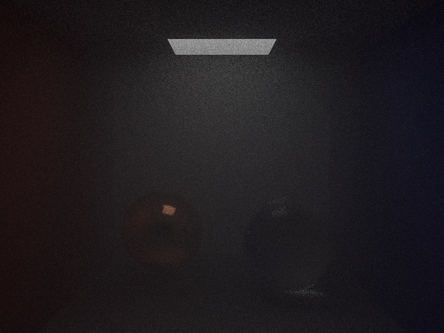
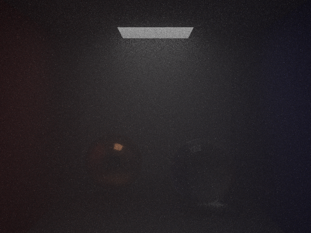
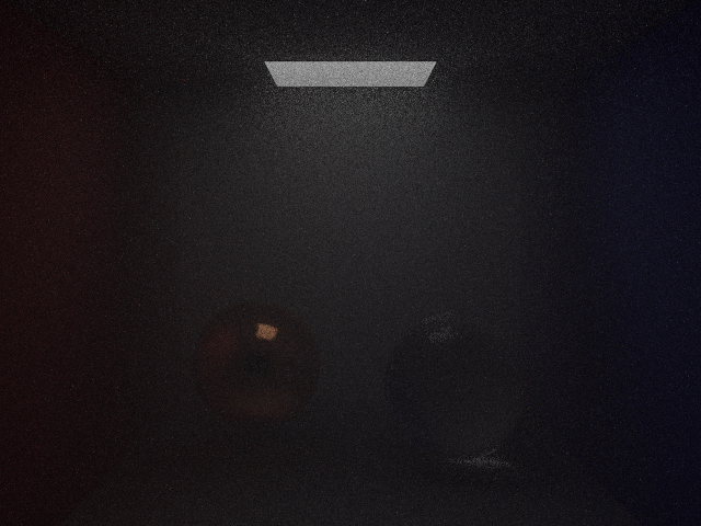
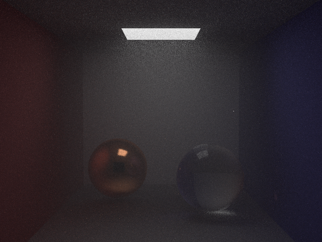
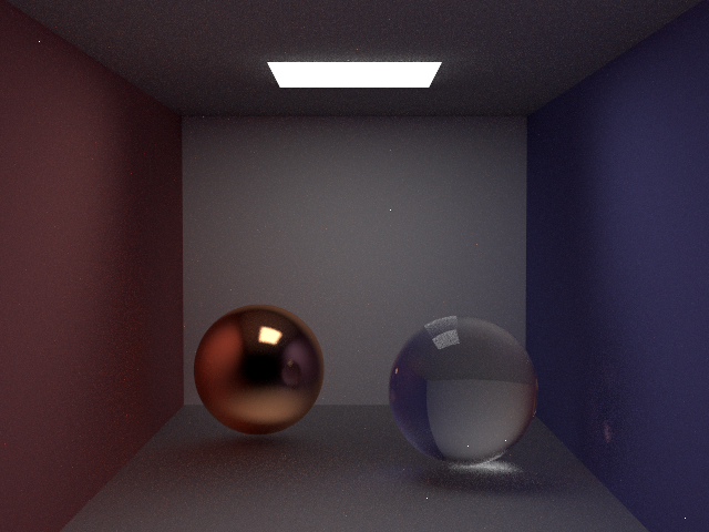
With no volumes:
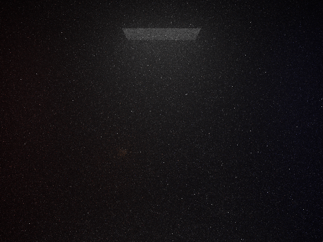
Volumes with various parameters:
According to
http://misclab.umeoce.maine.edu/boss/classes/RT_Weizmann/Chapter3.pdf,
a reasonable approximation for the inside of water is a medium with
g = 0.924, sigma_t = 2, sigma_s = 1.5.
Nee and MIS
Code: `src/integrators/path_tracer_volumetric.cpp`
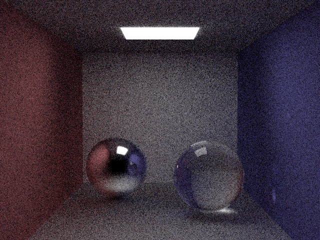
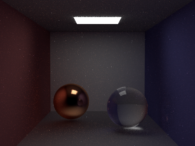
Our basic volumetric path tracer integrator yielded very noisy results, so we decided to add next event estimation and mixed importance sampling to our implementation.
Basic materials integration with volumetrics:
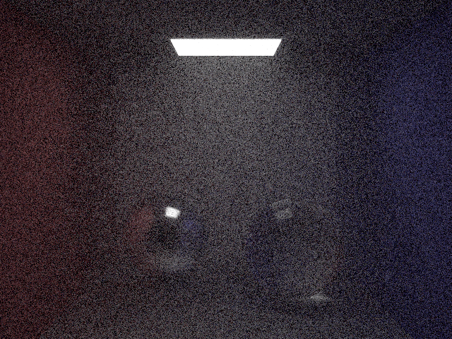
Code: `src/integrators/path_tracer_volumetric_nee.cpp`
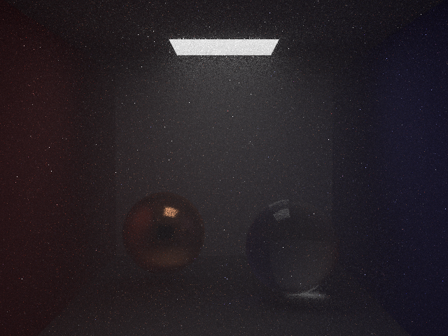
Adding only next event estimation caused the characteristic sparkly appearance in both volumetrics and regular materials:
Code: `src/integrators/path_tracer_volumetric_mis.cpp`
In our final MIS implementation, we importance sampled in the usual way for regular materials. For volumetrics, we took one random scatter sample and one sample in the direction of the light source. This results in a nice, fine-grained fog:
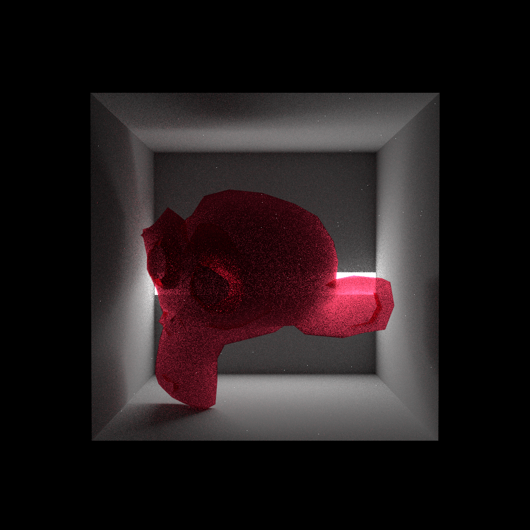
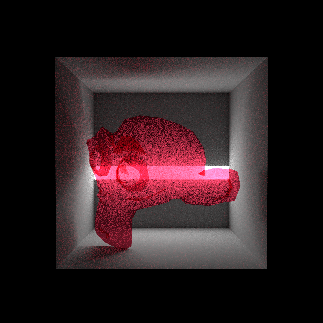
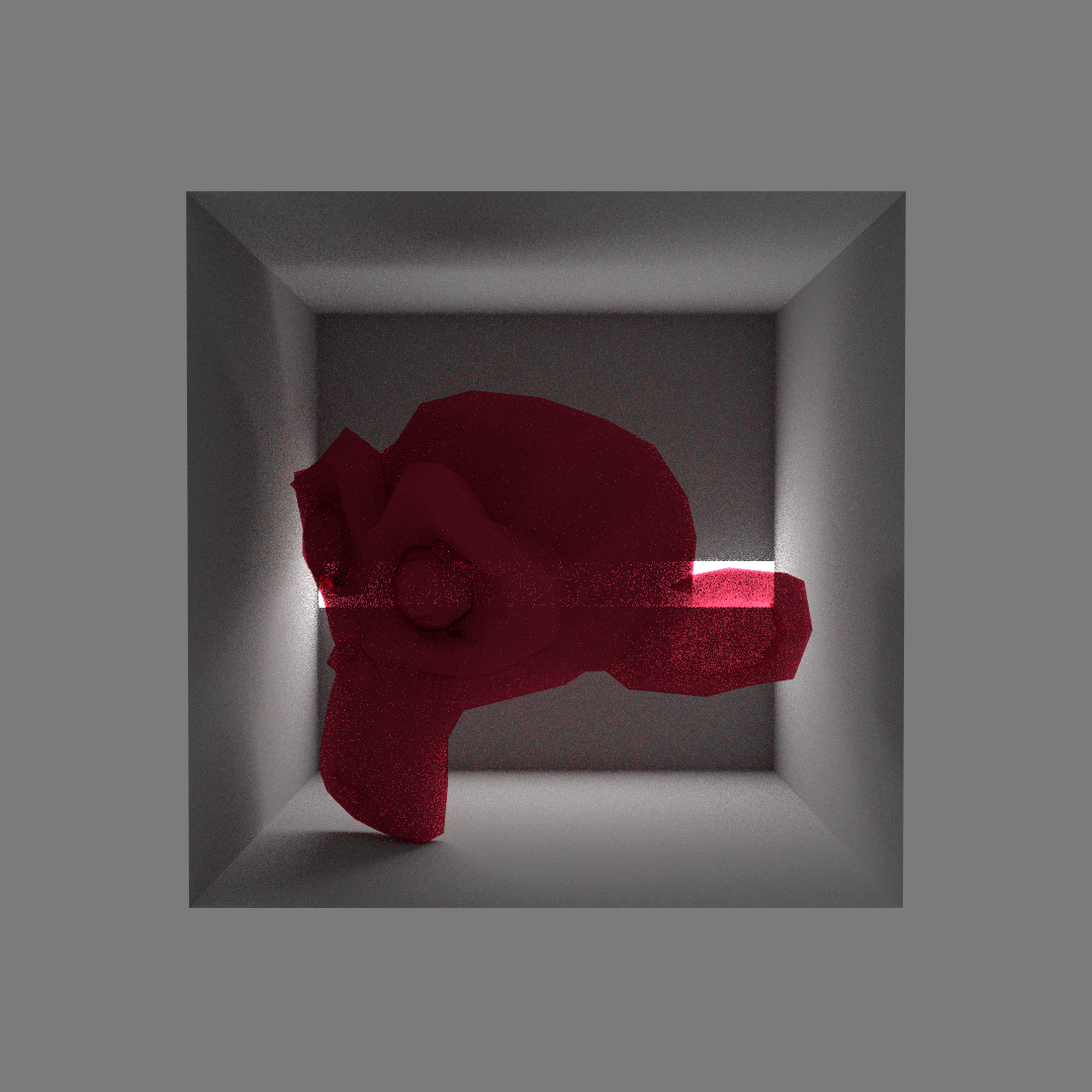
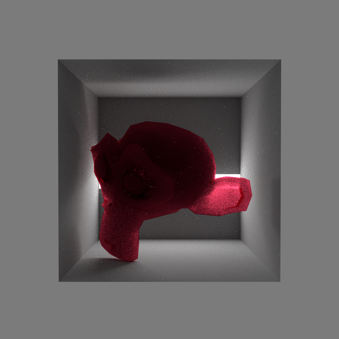
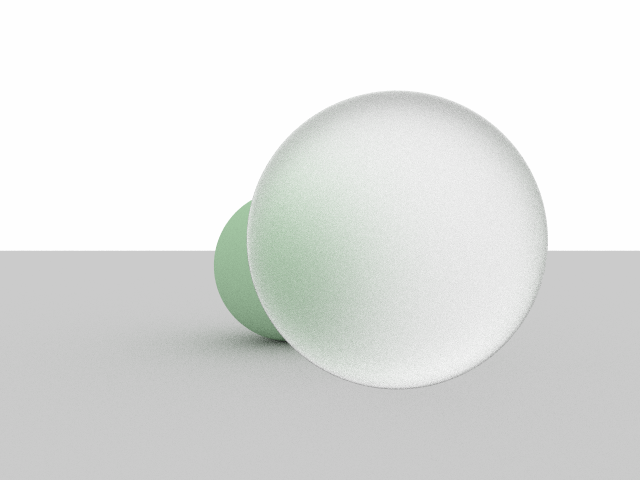
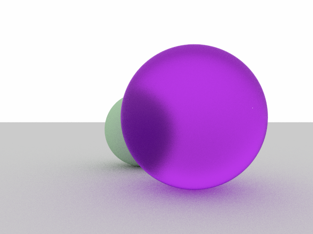
Non-exponential bleed (subsurface) medium
Code: `src/media/nonexponential_bleed.cpp`
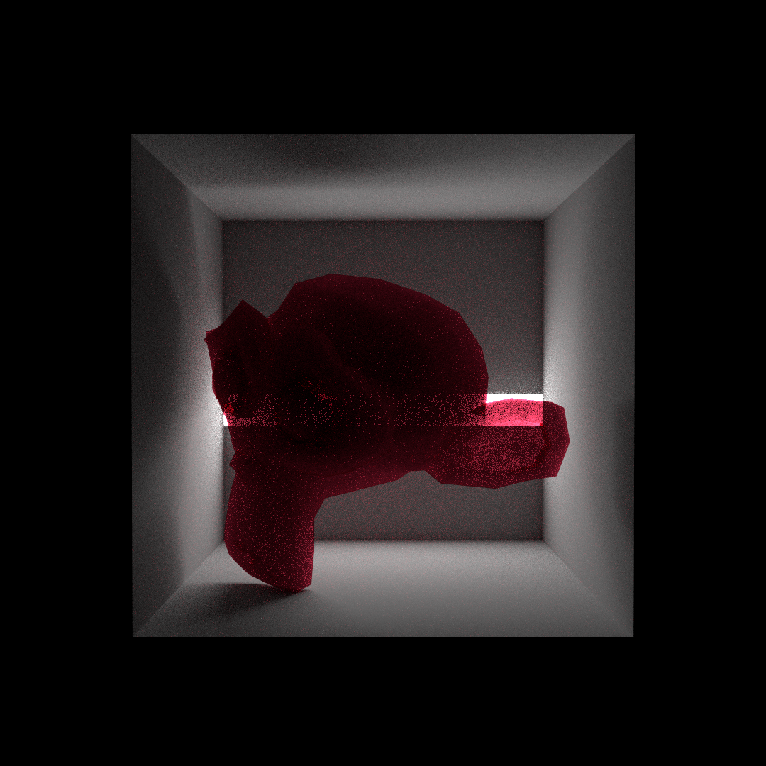
One way to simulate subsurface scattering is to place a volume with a very high scattering coefficient inside a surface boundary--while this is less efficient than a non-empirical diffusion approximation, which “provide a closed-form and accurate solution where the surface is flat, areas with high curvature (for example, the nose or ears of a human face) present a problem in that the semi-infinite slab approximation fails. If we instead consider the medium embedded in the surface to be just another volume, we can use the same path tracing technique for subsurface scattering as for general volume rendering.” (source https://graphics.pixar.com/library/PathTracedSubsurface/paper.pdf ) This paper also suggests a more physical, “non-exponential” approach to such a subsurface scattering volume; “As light moves through a participating medium, the proportion of unscattered to scattered light is a function of the distance traveled” (see section 7, Non-Exponential Free Flight). We implemented a non-exponential free-flight media wherein, as opposed to the homogeneous Henyey-Greenstein medium in which “the probability of scattering is proportional only to the scattering cross section of the medium,” the “probability . . . becomes a function of both the scattering cross section as well as the distance traveled in the medium.” Built into the paper’s nonexponential medium was also a “bleed” parameter, which we implemented to allow the user to control the degree to which light penetrates the SSS medium. The higher the bleed number, the greater the penetration.
Results:
As you can see, the `g` parameter, which determines forward or backward scattering in relation to the light source, greatly changes the look of the medium. With lower bleed parameter:
Straight Line Hack
To improve rendering of SDS paths for underwater objects, we decided to introduce a non-physical hack where shadow rays, when refracting through
a dialectric, continue in their original direction instead of the true refraction direction.
This makes it so that the traced shadow rays actually reach the light source --- especially if the light source is small or far away.
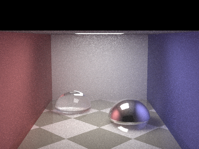
Below is a test of the straight line hack to improve visability of a checkboard texture below a dialectric plane:
In the above example, we see that the ground became a good bit lighter --- which we think is due to more shadow rays actually reaching the light source ---
while the walls became a bit but less lighter, due to extra indirect lighting.
This work is implemented in the integrators at
`src/integrators/path_tracer_volumetric_nee_hack.cpp` and
`src/integrators/path_tracer_volumetric_nee_mis.cpp`.
Anisotropic BSDF approximation
One feature of selenite, or more correctly "satin spar", is that it is chatoyant.
https://66.media.tumblr.com/0d9ab0ea7ff630fbb5326eb5bc53403d/tumblr_prgjrk2n2h1st8h25_1280.jpg
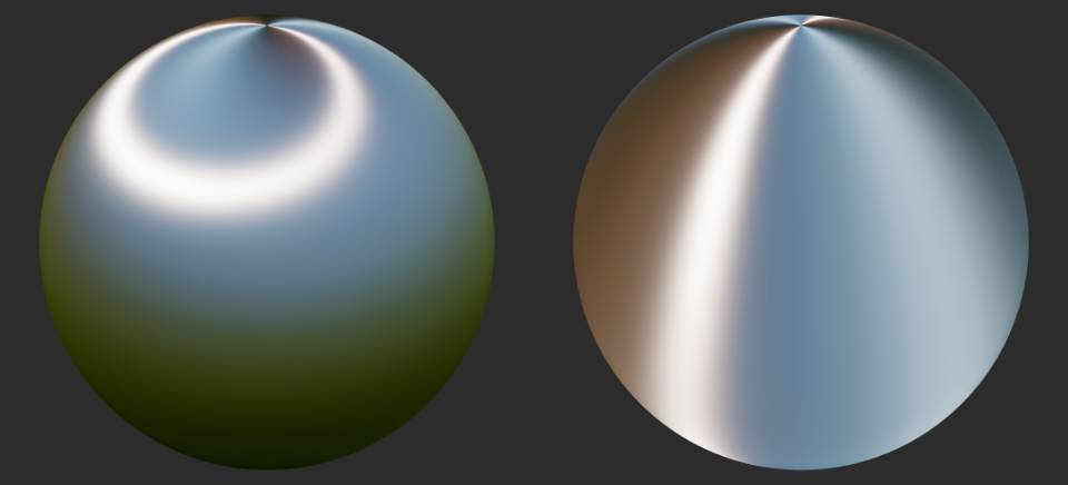
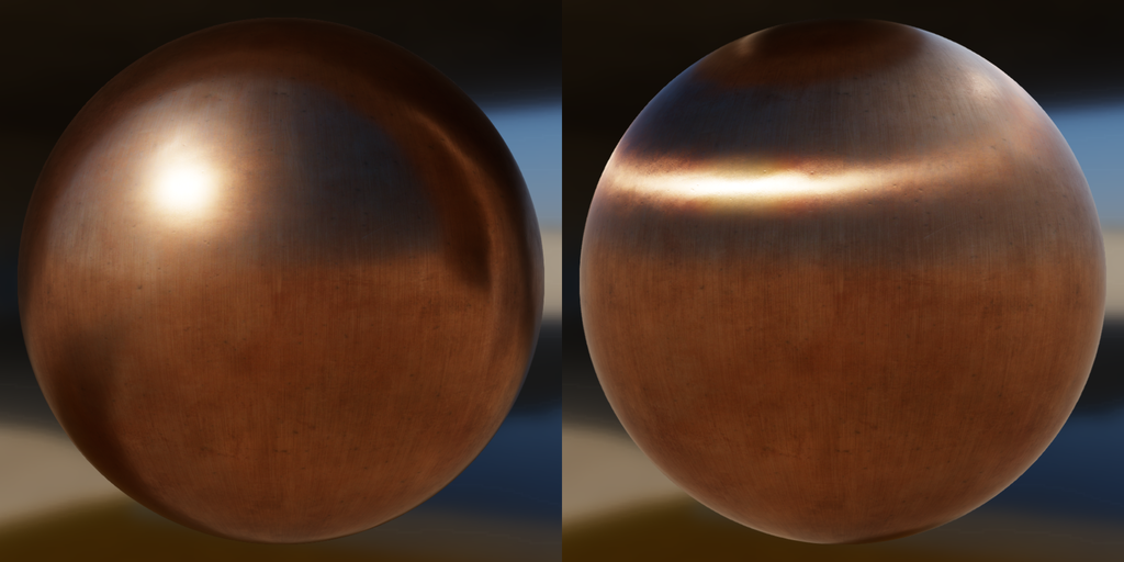
We found an anisotropic bsdf described in the Filament renderer documentation which
seemed able to approximate this effect -- here are two of their reference images:
https://google.github.io/filament/Materials.md.html#materialmodels/litmodel/anisotropy
https://google.github.io/filament/Filament.html#lighting/imagebasedlights/anisotropy
Their approach uses tangent and bitangent vectors to form a "bent normal" vector which the incoming ray is then reflected about.
As the anisotropy parameter varies, the specular highlights aligns more towards either the tangent or bitangent vectors.
We adapted their approach to construct a anisotropic dialectric, which, on reflection, behaves like the Filament anisotropic material,
and behaves like a usual dialectric on refraction. To make the tangent and bitangent vectors make sense for a crystal, we made it so that the tangent
direction was as "upward" as posible in the tangent plane to the shading normal, where "upward" is the direction the object or crystal is pointing,
and which must be entered into the json file. See `src/materials/anisotropic_dialectric.cpp` for our implementation.
Here are some examples of our anisotropic dialectric:
Because we were not able to replicate the brushed metal reflections above, we are not confident that this anisotropic material is working properly,
but it does seem to generally warp reflections in the appropriate direction as anisotropy is varied.
Rough Dielectric Material
We had a few motivations for making a rough dialectric material.
One was to potentially use it for our water surface to avoid SDS paths, and another was that
it might be a good model for our crystal surfaces.
We implemented this material by layering the cosine lobe idea from the Phong BRDF on top
of the reflection and refraction directions from the dialectric. In more detail, the rough dialectric
sample decided whether to reflect or refract in the same way as the standard dialectric, then used
our orthonormal basis structure to sample a cosine lobe around the usual reflection/refraction direciton.
The pdf for the sample was then scaled by the reflection/refraction probability.
See `src/materials/rough_dialectric.cpp` for the impelmentation.
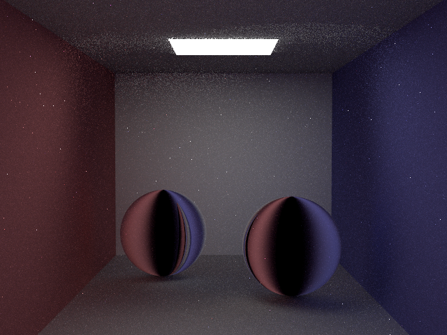
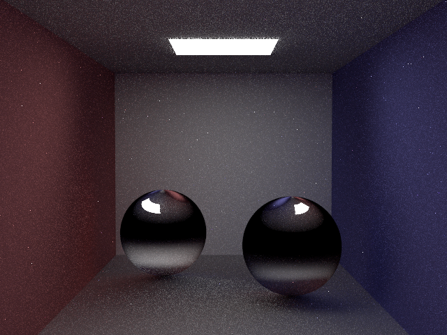
Here are some examples of the `04_refr` scene with different cosine exponents:
As the cosine exponent tends to infinity, we expected the rough dialectric to approach the usual dialectric:
It takes a surprisingly high exponent to get rid of noticeable blur!
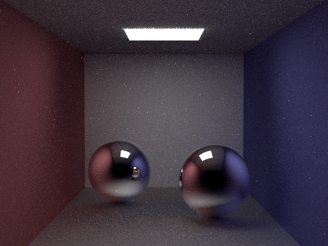
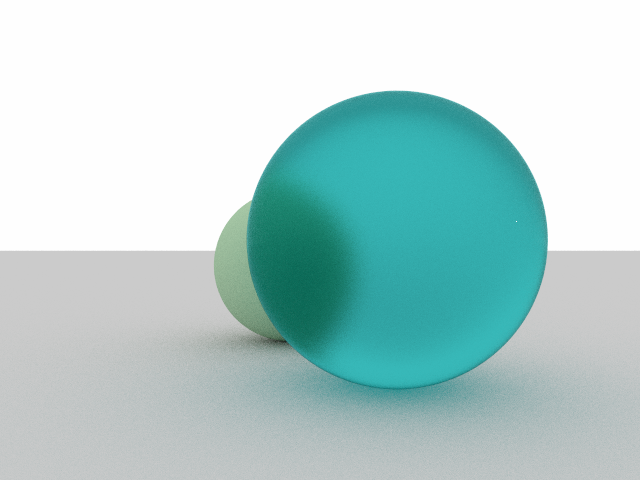
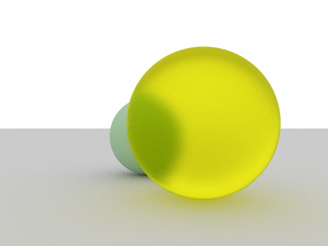
We also modified the rough dialectric (and all our specular materials) to take a color scatter parameter.
Our reference for this was
https://google.github.io/filament/Materials.md.html#materialmodels/litmodel/absorption.
Here are some examples tinting the rough dialectric different colors:
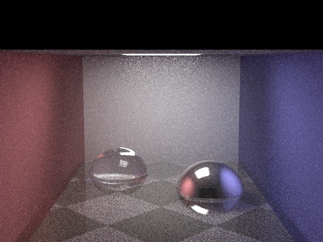
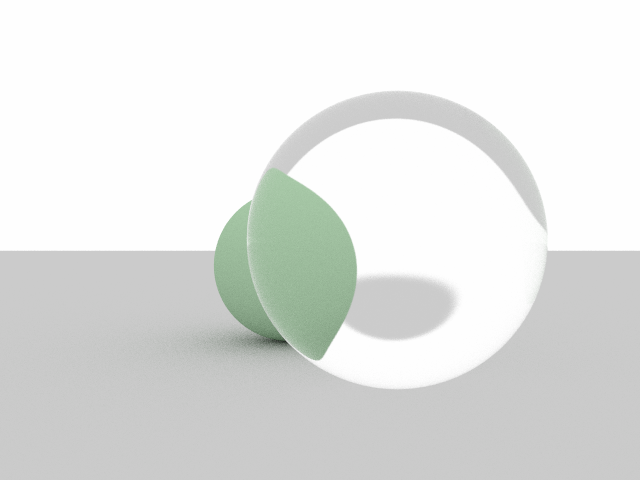
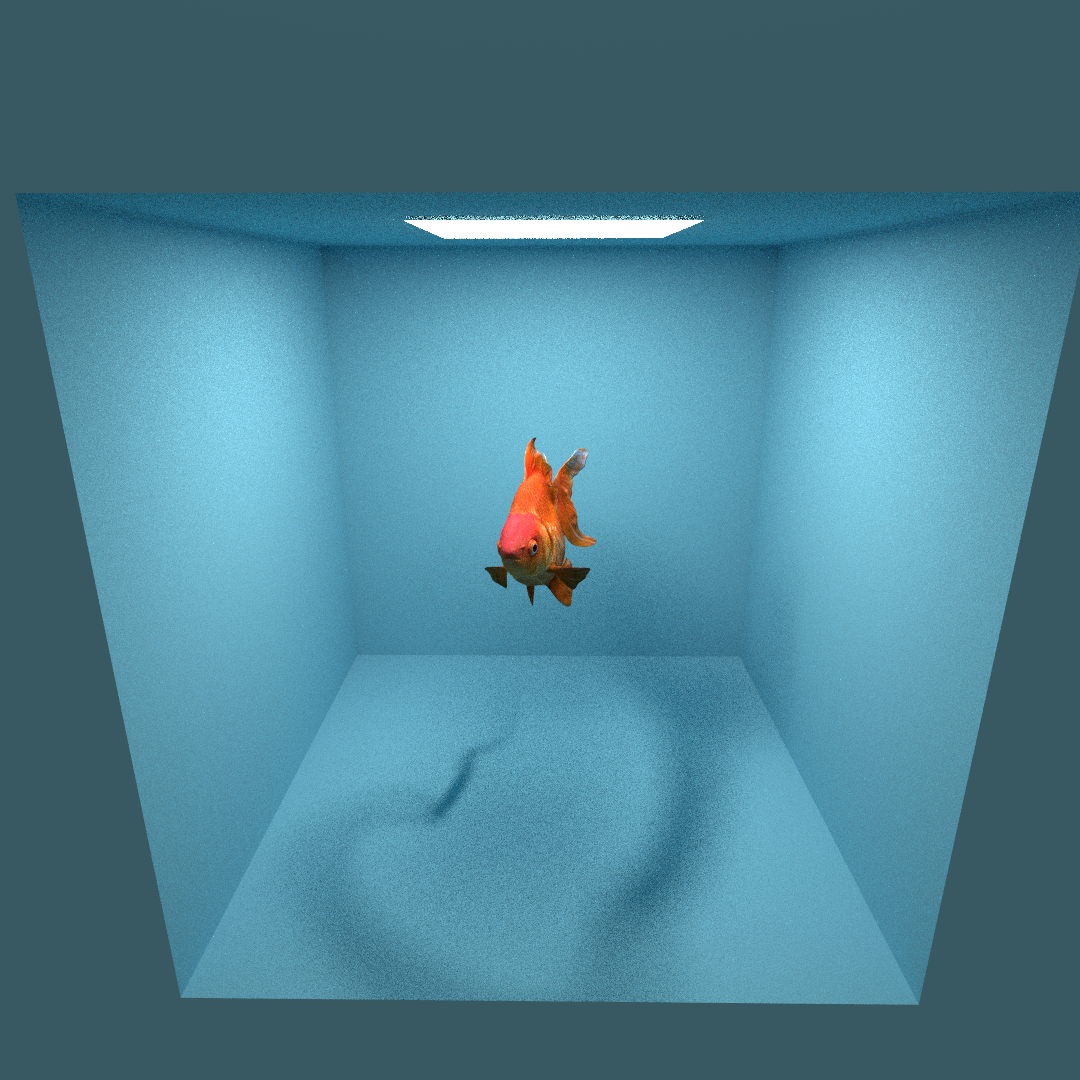
“Invisible” and “Substitute” Materials
To render a fish casting a dragon shadow, we had to figure out how to create an “invisible” surface that also occluded (the dragon),
as well as a “substitute” material (the fish) which would be visible but not occlude. To do this, we added the boolean fields `is_invisible`
and `is_substitute` to our surface base class, as well as a `hit_invisible` parameter to our `Li_helper`.
Shadow rays were traced with "hit_invisible" set to false, and all other rays with it set to true. When a `hit_invisble = false` ray hit an invisible material or
a `hit invisible = true` ray hit a substitute material, the ray continues as if the surface wasn't there by a recursive call to `Li_helper`.
Any other surface intersections are treated as usual. You can see this process in `src/integrators/path_tracer_volumetric_nee_mis.cpp`.
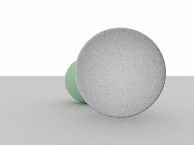
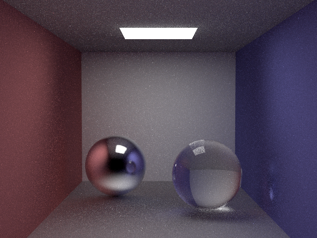
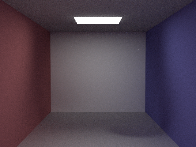
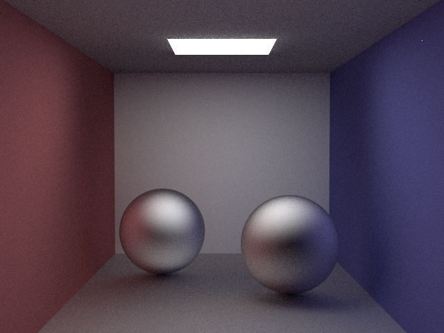
Here is an example showing invisible spheres in the Jensen box:
Note in the above that the shadows cast by invisible surfaces do not depend on the surface material,
and that effects such as the increased shadowing near touch points (due to occluding of non-shadow rays)
do not appear when the surfaces are made invisible. Our straightforward approach using shadow rays, though,
gives the dragon shadow effect we wanted.
Another neat thing is that, for an invisible surface in media, one can decide whether or not the invisible surface
casts a volume or just a surface shadow by changing the "hit_invisible" parameter for volumetric shadow rays.
Other Timesinks
K-D Tree
We were hoping to implement photon mapping to give better crystal caustics and avoid the straight-line hack.
We unfortunately didn't get this running, but we did code (from scratch) and test the key data structures:
the k-d tree with k nearest neighbors and the max heap to speed up nearest neighbor search.
The implementation is located in `include/darts/kdtree` and `src/kdtree.cpp`, and the testing file is at `kdtree_test.cpp`.
Here is an test run where we build a photon map from 1M randomly generated photon positions, note that the the other photon parameters are set to 0.
To make this work, the stack limit must be expanded (`ulimit -s 32000` works), and I had to work in terminal (not vscode) to effect this stack change.
The data structures are quite fast, and the following test with 1M photons just takes a second or two:
We mostly paired-programmed our features, though a few were either implemented
or designed/prepared independantly prior to a joint programming session.
Items besides the following were programmed together.
Matt
did k-d tree and related structures independently
prepared and designed rough dialectric
Leah
did non-exponential bleed independently
prepared anisotropic bsdf
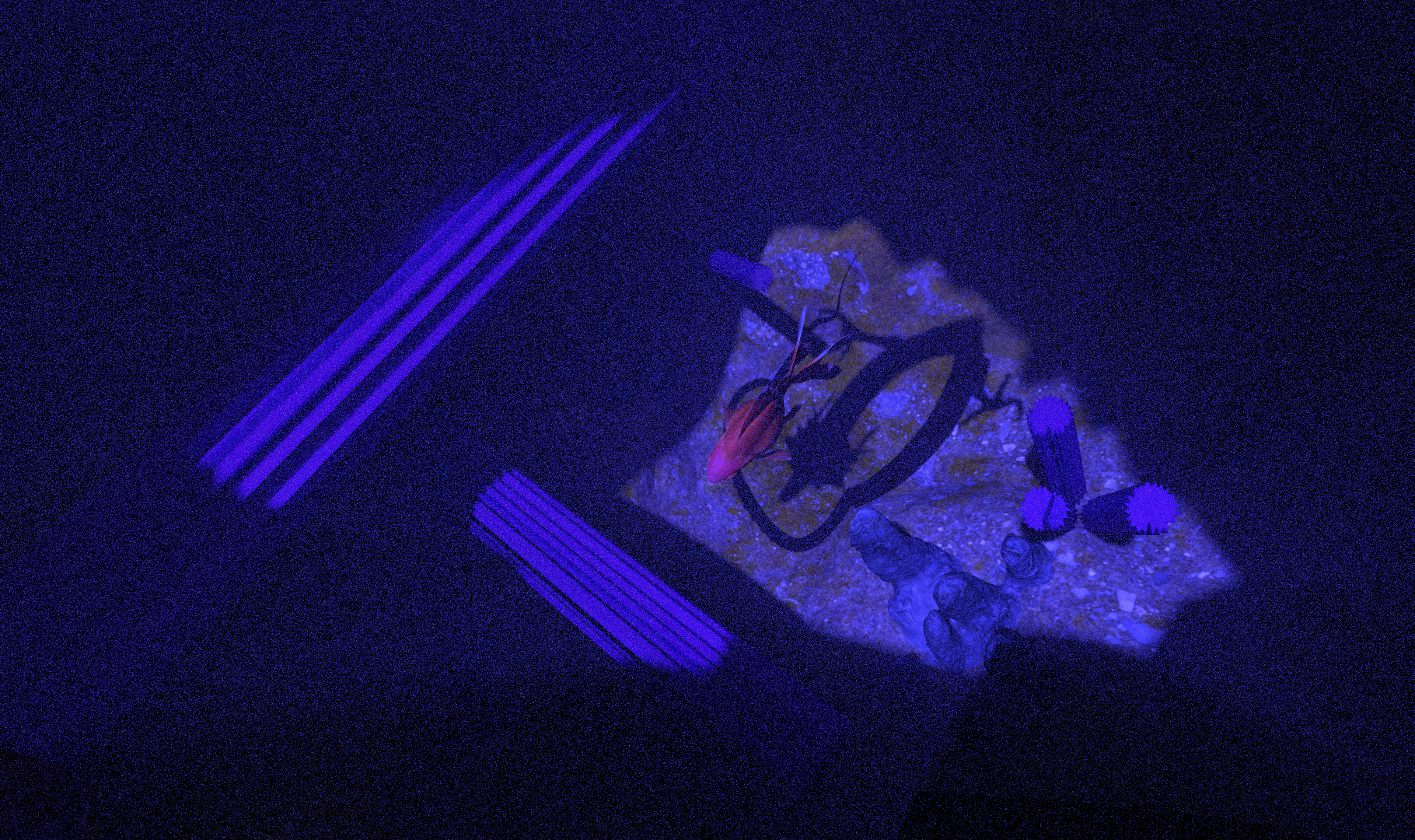
Final image
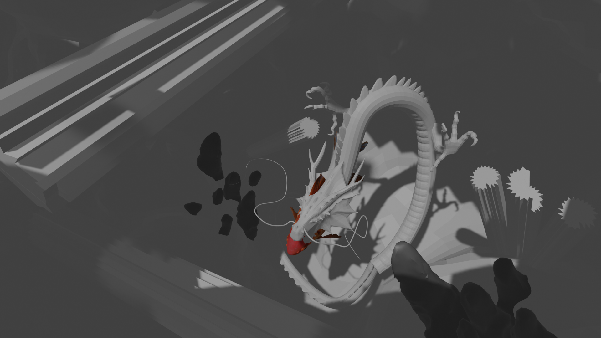
Scene rendered in Blender (example shot):
We weren't able to use the Discovery cluster to render our images because the EXR outputs from the cluster looked very different from those rendered on our local machines. Despite spending a couple of days on these bugs, which in no small part were being caused by uncaught NaNs (when dividing by zero PDFs) and by Discovery's disparate `abs()` function, we were unable to get the EXR Discovery images to match our local references. Having rendered our final scene on several different machines with different seeding and averaging the results, this is the final image:
 Volumes with various parameters:
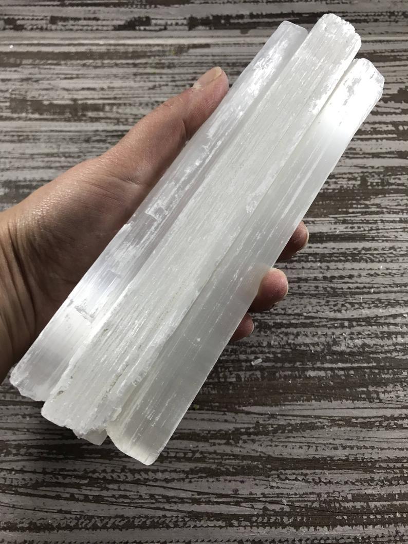 https://66.media.tumblr.com/0d9ab0ea7ff630fbb5326eb5bc53403d/tumblr_prgjrk2n2h1st8h25_1280.jpg
We found an anisotropic bsdf described in the Filament renderer documentation which
seemed able to approximate this effect -- here are two of their reference images:
https://google.github.io/filament/Materials.md.html#materialmodels/litmodel/anisotropy
https://google.github.io/filament/Filament.html#lighting/imagebasedlights/anisotropy
https://66.media.tumblr.com/0d9ab0ea7ff630fbb5326eb5bc53403d/tumblr_prgjrk2n2h1st8h25_1280.jpg
We found an anisotropic bsdf described in the Filament renderer documentation which
seemed able to approximate this effect -- here are two of their reference images:
https://google.github.io/filament/Materials.md.html#materialmodels/litmodel/anisotropy
https://google.github.io/filament/Filament.html#lighting/imagebasedlights/anisotropy


 We weren't able to use the Discovery cluster to render our images because the EXR outputs from the cluster looked very different from those rendered on our local machines. Despite spending a couple of days on these bugs, which in no small part were being caused by uncaught NaNs (when dividing by zero PDFs) and by Discovery's disparate `abs()` function, we were unable to get the EXR Discovery images to match our local references. Having rendered our final scene on several different machines with different seeding and averaging the results, this is the final image: