Analysis

Figure 4: Simple Good-Turing smoothed $n$ -gram probability mass for {1,2,3}-grams. Notice how each log-log plot contains a smooth line, masses are concentrated in lower frequencies $i$ as $N_i$ increases, and reserved probability mass increases with the $n$ -gram size. The last point suggests larger $n$ -grams are very sparse. We do not have sufficient examples to see many new $n$ -grams, and even if we had them, grammatical correctness would limit the number of new $n$ -grams.

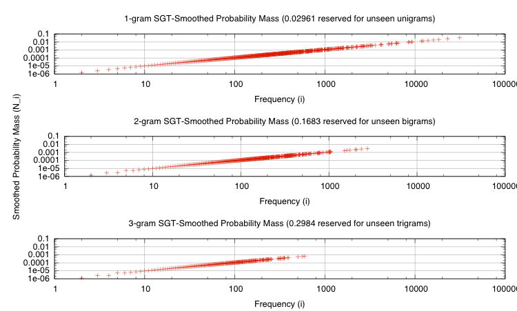Figure 5: Word prediction performance using unigrams and bigrams. We define ``hit'' to mean a correct word prediction, ``miss'' to mean an incorrect prediction, and ``near hit'' to mean that a matching bigram existed, but wasn't chosen because it didn't have the highest smoothed probability. The plot depicts the mean hit rate as $\approx 29\%$ and the mean near hit rate as $\approx 71\%$ . We computed these values over our entire dataset after smoothing $n$ -gram probability mass using SGT.

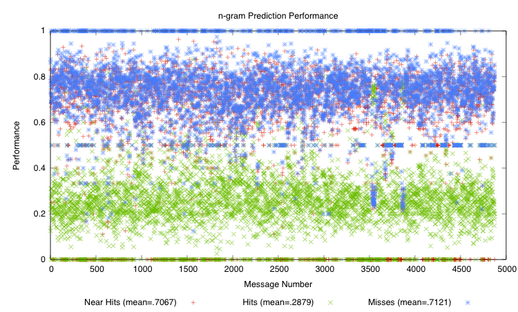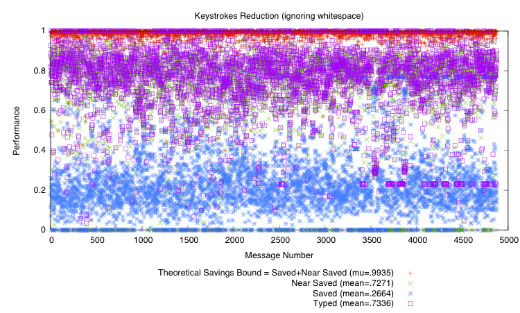
Figure 6: Keystroke reduction using unigrams and bigrams, not counting whitespace. We define ``saved'' to mean a correct word prediction that eliminates typing; ``typed'' to mean characters typed by the user because of an incorrect prediction; and ``near saved'' to mean that a matching bigram existed, so typing could have been avoided, but the system didn't choose the bigram because it didn't have the highest smoothed probability. The plot depicts the mean savings rate as $\approx 27\%$ and the mean near save rate as $\approx 73\%$ . We computed these values over our entire dataset after smoothing $n$ -gram probability mass using SGT. We may find a lower ``near save'' when we split the dataset into training and testing portions.

Here, we apply the C-based SGT estimator to unigrams, bigrams, and trigrams from the entire dataset and subsequently compute word predictions using a python script.

Figure 4 depicts the probability mass associated with each these $n$ -gram dissections of the dataset, Figure 5 shows word prediction performance using estimators derived from unigrams and bigrams according to equation (2), and Figure 6 shows keystroke reduction as a result of correct word prediction. We have not yet analyzed performance after splitting data into training and testing sets, nor have we analyzed the effects of trigrams on prediction performance. We plan to take these steps later.

To gain a sense of performance, we have smoothed the entire dataset and computed hits, near hits, and misses for each message. A hit is the number of times a correct prediction is made; a near hit means that a bigram existed, but it wasn't chosen because it did't have the highest smoothed probability; and a miss is the number of incorrect predictions.

Overall, the mean of bigram performance is approximately $29\%$ and the mean of the near-hit rate is closer to $71\%$ . Assessing trigram performance, perhaps combining the two, and using context such as the next typed letter might lead closer to the upper-bound performance depicted in the plot. In the upper bound, we assume an ability tob convert all near hits to hits.