Team Members
Ruzi Zhang
Shiyuan Jiang
Yibo Long
Introduction
Recommending movies can be based on various biases. Most recommender systems(RS) are based on users’ social connections or ratings. Some others use keyword context and time to filter related movies.
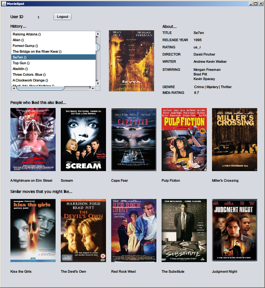
MovieSpot is a movie recommender system integrated with both social information and movie contents. It is also the first movie RS equipped with an learning model of visual features. It provide us a way to criticize a movie that has never happened before.
This idea came from the inspiration of the movie barcode, which compresses a movie into colorful and elongated barcode.

Because of the difficulty in generating barcode, we used posters instead as the visual element in the project. We implemented our integrated recommendation approach as a Java application which shows directly the effectiveness of our method compared with the social-only system.
Methods
A complete RS should include the prediction from both content and social ratings of a movie. So we will build our system on both tracks, and evaluate whether it helps to improve the recommendation. But most importantly it provides us a way to criticize a movie that has never happened before.
Through content-based RS we try to evaluate a whole movie in every aspect. If it can even go through a whole movie to make a criticism, it will become an expert. That’s why we hold a high expectation of visual element like barcodes and posters.
Therefore, the comparison between content-based and social RS is not only for building a hybrid RS, but also for finding and learning what entertains audience most. A strong recommendation from content-based methods differs from social-based one may suggest that some elements are less important for recommendation and may also suggest that the director should shift his attention to other points that attract audience.
We will firstly present our algorithms in two system, then list the evaluation criteria that we use to make the comparison.
Content-based Recommender System
A content-based recommender system takes advantage of social ones as it merely needs context to make a prediction. When problems comes to rare movies or new movies, insufficient ratings and comments fails to make a difference. However, lacking sociality makes it difficult to personal recommendation, but avoids the problems a social RS has, such as, data sparsity, scalability, cold start[12].
Movie Representation
The content of a movie will be presented by a vector space. Following features are included in our system.
Content
There are many contents that we think help contribute the recommendation[7], like title, genre, director, actors, plot keywords, etc. We try to pick up features that present what a movie is rather than that help predict the rate. These features like poster may indicate the taste of a movie but cannot be enough to predict what the rate of a movie is.
As a job of finding the similarity of movies, we believe these features with poster features are more suitable. Other features most content-based RS use, like user comments, reviews should be better for the goal of predicting rate.
Poster
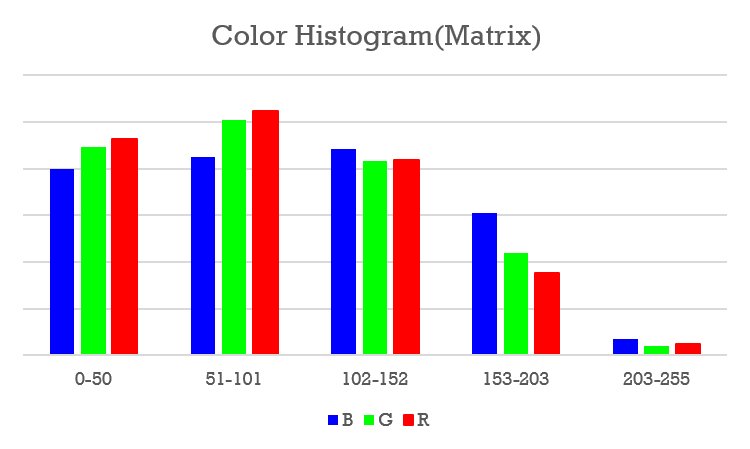
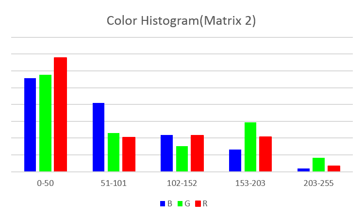
After researching, we found a sparse representation based on bags of visual words[6][10] is highly suitable. An image can be represented as an array of integers using this methods. Each image is divided into square blocks, and each block is represented by color or edge histogram. By counting the block in a predefined set(dictionary) of d = 10,000 vectors of such features, the image is thus represented as the frequency of limited blocks.
Though it is not like the barcode feature we mentioned before, the poster still captures one’s eyes by emphasizing sale points and the mood in the scene. Therefore, histogram can be helpful to present those in blocks. These features were systematically tested and found to outperform other features in related tasks[2].
We chose 5 bins in for the color histogram, and 5 types of edge descriptor.
The edge descriptor is first implemented in this paper[13]. 5 types of edge are categorized as: vertical, horizontal, 45-degree diagonal, 135-degree diagonal, and non-directional edges
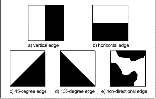
we use coefficient filtering to calculate these edges. the coefficients are defined as follow:
| 1 | -1 |
| 1 | -1 |
| 1 | 1 |
| -1 | -1 |
| sqrt(2) | 0 |
| 0 | -sqrt(2) |
| 0 | sqrt(2) |
| -sqrt(2) | 0 |
| 2 | -2 |
| -2 | 2 |
These features can describe the texture of an image, and help find the similarity in local areas.
We tried to implement Pyramid to build a multi-scale representation. Such model is helpful when we abstract the image into sub-images.
Local Discriminative Distance Metrics Ensemble Learning
The recommendation result will then be computed based on k-nearest-neighbor, the similarity between movies can be calculated by Euclidean distance.
But the poster’s feature occupies most of the attributes of a movie, which heavily influences the judgement based on the those features. This is not what we want to see either for predicting rate or recommending similar movies.
We want to learn a weight by Metric Learning. As the Euclidean distance can be expressed as follow:

For a new function for input x F(x)=Lx , the distance function can be expressed as

The Metric Learning’s goal is following:[14]

A global approach of the metric may not be suitable for the whole problem, so we use a local metric learning method to help build the system. A local metric system is also more suitable to recommend movie for individual users since the metric is learnt by the user’s history.
Local Discriminative Distance Metric(LDDM) is a multiple metrics approach that is demonstrated to outperform other methods. It has a objective function similar to other metric learning method.

Where  is the focal sample for local learning,
  is the sample from the same class,
  is the sample from different classes,
  is the metric distance that we want to learn,
  is a multiplicative factor to balance the influence of equivalence constraints and inequivalence constraints with respect to the focal sample.
According to the definition, it can be reduced to:

Where  ,
,  ,
,  is the jth column in the focal vicinity matrix
  .
.  is given by

To make the projection metric learned from the local vicinity linear and orthogonal, we impose  , then it is deformed to

The solution to this can be obtained with the standard eigendecomposition.
A local metric can also be obtained from the history of a user, the procedure is following:
- find the focal sample that is closest to the center of the samples
- sort the samples based on the distance to the focal sample
- make the first half the samples close to , and the rest away from
- learn the LDDM with the local vicinity.
We use classifiers ensemble learning for the multiple metrics. The local classification is a probabilistic approach. To predict the class label o of sample  with focal sample , the probability of belonging to the class o
  using the local distance metric
  is
is

where  is an indicator function that returns 1 when the input argument is true, and 0 otherwise.
Note that if we use only part of the samples to build the focal, the overall test time of LDDM is even faster than KNN. As the author mentioned, the training and testing phase can be parallelized to make it scalable for large-scale problems.[18] Local classifiers could also be learned offline in advance, and updated when new samples are added.
This paper also made a theoretical analysis of LDDM. it proves the convergence rate bound, the generalization bound of the local distance metrics and the final ensemble classifier.[18]
We then use voting method for the ensemble learning.
The parameters of LDDM are k1, k2, and k. k1 and k2 are set to 200 according to the author’s analysis. We will test the k’s influence on the result.
Social Recommender System
Social recommender system is usually based on users’ rating and connections. The social network or similar users who have the similar history provide the evidence of recommendations.
Collaborative filtering (CF) is a technique aimed at solving this problem[3]. There are two models are based on CF. User-based collaborative filtering predicts a test user’s interest in a test item based on rating information from similar user profiles. Item-based collaborative filtering otherwise uses similarity from items as the basis.
The algorithms we use are all based on KNN, one is Item-based, another is User-based.
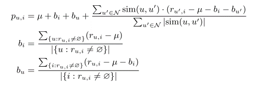
The basic idea of item-based CF is to compute similarities between items, typically based on the users that have rated them, and the recommend items similar to the items that other user likes. The similarity equation between item i and item j in our system is express as follow:[15]

User-base CF is also tested in our system. We implemented item-user mean normalization for prediction, resulting in the following prediction rule (is the global mean rating, N the most similar users who have rated i, and ru,i=for missing ratings):[16]
Evaluation Criteria
RMSE
The root-mean-square error (RMSE) is a frequently used measurement of the differences between values predicted by a model or an estimator and the values actually observed. These individual differences are called residuals when the calculations are performed over the data sample that was used for estimation, and are called prediction errors when computed out-of-sample. The RMSE serves to aggregate the magnitudes of the errors in predictions for various times into a single measurement of predictive power. RMSE is a good measurement of accuracy, but only to compare forecasting errors of different models for a particular variable and not between variables, as it is scale-dependent.[17]
The RMSE is tested on the same criterion. For every item, RMSE is calculated between the predicted rate and the actual rate. Therefore, this result is rate related.
Quality
The quality of the recommend movies refers to the average rating from IMDb users to the recommend items to certain movie. This measurement reflects how well accepted by the public are the recommend items. It is also a rate related criterion.
Overlap rate
The overlap rate is defined as the proportion of same recommended items in two systems. This measurement can be helpful to find the similarity of two RS. Lower rate indicates the set of recommendation is almost orthogonal, otherwise the recommendation is similar to each other.
Individual case
We observe the recommendations of certain movies under different methods and try to figure out similarity and difference of those results.
We believe this is necessary because what users really think as a good recommend is not rate related.
Dataset
Our social rating subsystem is based on dataset provided by GroupLens Research Project at the University of Minnesota. It contains 100,000 ratings (range from 1 to 5) from 943 users on 1682 movies, and each user has rated at least 20 movies. It also simplifies the demographic info for the users as a tuple of age, gender, occupation and zip.
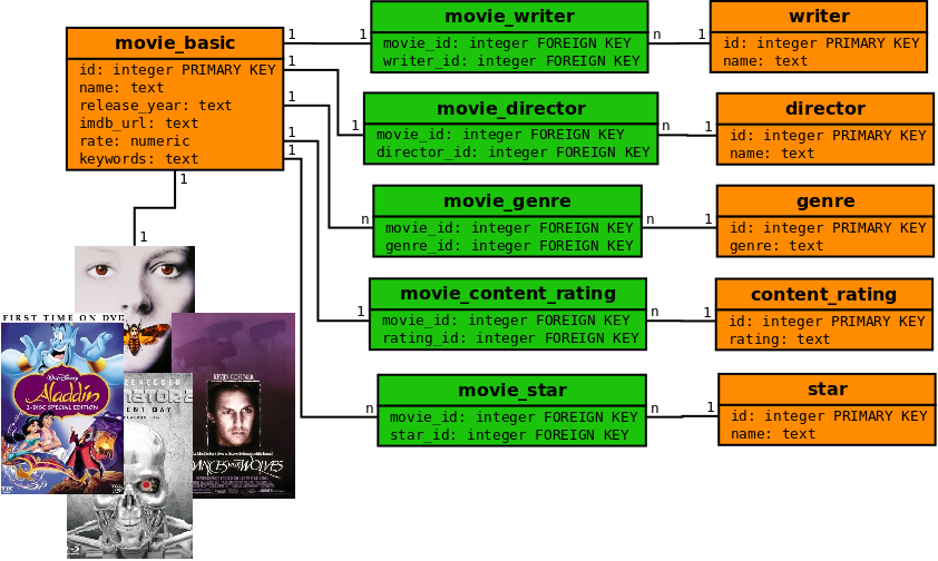
For the content-based subsystem, we collected central movie content information (poster, release year, average rating, plot keywords, director, writer, starring, genre and content rating) of the 1682 movies in Grouplens dataset from IMDb. Since posters are significant features in our recommendation strategy, we cleaned up all movies that have no poster on the website during data fetching process, reaching a dataset of 1628 movies. To make our life easier, we store 1 director, 1 writer and at most 3 actors, which are more important than the rest movie features for each movie.
As mentioned above, some attributes, like starring, genre and keywords, have multiple values. To speed up our system, for starring and genre that are comparatively more important and have less possible value, we store them with relational approach, while for keywords we store it as a long text and separate each word with comma.
We also adopt a simple method to access poster data --store poster with a filename format “movie_id.jpg” and construct that filename when needed.
Figure 6 shows the association between features and movies in the relational database.
Results
RMSE
Figure 7 shows the RMSE of the four methods.
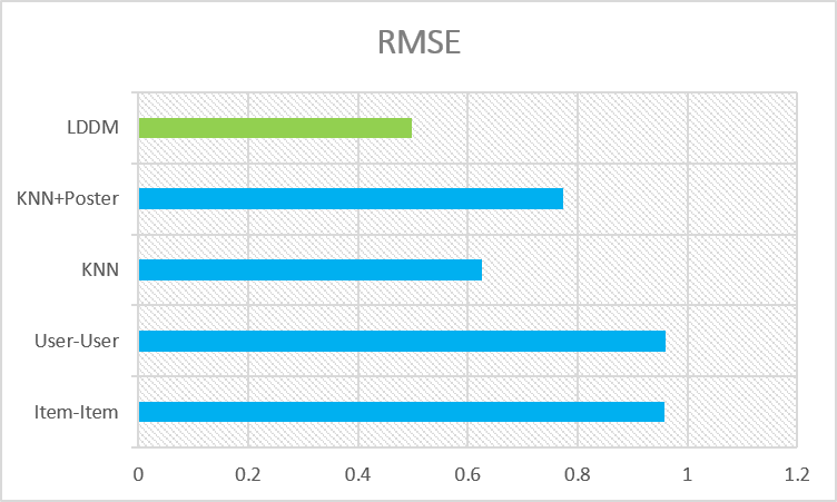
As the RMSE of the KNN is smaller than that of the KNN+Poster, this result indicates that the large scale of features, which are extracted from the posters, may not improve the score prediction. Also, the RMSEs of both of the second two methods are smaller than those of the last two methods, showing that the content based RS performs even better in this measure. Also, the LDDM approach has least RMSE, indicating a best rating predictor.
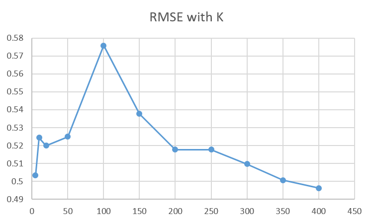
the author of LDDM set the K based on empirical observation. The result is based on k1=200, k2=200. We can see LDDM is not very sensible to the parameter K. k1, k2, and have more influence on the learning result.
Quality
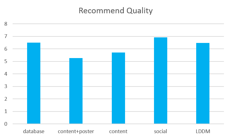
The second result is shown in Figure 9. In this phase, the quality of the social based RS outnumbers that of the content based RS. This means that more accepted good movies are recommended by the social based RS than the content based RS. In addition, taking advantage of both two RSs, the LDDM approach has relatively high quality of items recommended and favors movies with similar poster fashion. We are able to see this advantage more clearly in the individual case afterwards.
Overlap rate
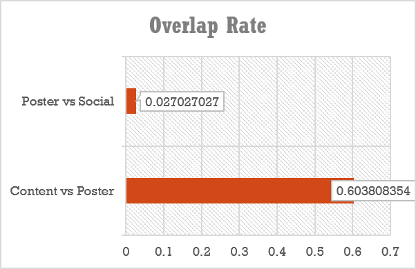
The low overlap rate of the content-and-poster based RS and the social RS shows that they rarely recommend the same movies, indicating different recommendation focuses. At the mean time, only 60% overlap rate of the content based RS and content-and-poster based RS reveal that posters’ features influence the recommendation result heavily.
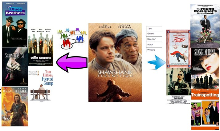
Individual case
Figure 11 illustrates the top 5 recommendations of the movie, The Shawshank Redemption, which is the TOP 1 movie of IMDB all the time. The recommend movies of the social based RS are The Blues Brothers, The Usual Suspects, Schindler's List, Forrest Gump and Braveheart. The recommend movies of the content based RS are Fargo, Taxi Driver, Yao a yao yao dao waipo qiao, The Young Poisoner's Handbook and Trainspotting. This also shows that the two RS have different recommendation focus. The social based RS is more likely to vote for the renowned movies of the same decade, whereas the content based RS tends to recommend movies with similar genre, taste and performance style. This is reasonable because users who have watched the TOP 1 movie rarely miss the TOP 10 list, while the recommendations of the content related RS cross the era and rate.
Another individual case is recommendation for Psycho, a 1960’s old horror movie.
| RS | Item | Recommendation | ||||
|---|---|---|---|---|---|---|
| Social | Psycho | Taxi Driver | The Blob | Ed Wood | The Godfather | Night of the Living Dead |
| Poster | Psycho | Phantoms | Lord of Illusions | Body Snatchers | Nightwatch | Rear Window |
| Content | Psycho | In the Mouth of Madness | New Nightmare | Lord of Illusions | The Relic | I Know What You Did Last Summer |
The result of social RS is becoming confusing. Taxi Driver, Ed Wood and The Godfather is obviously not horror movie, Ed Wood is surprisingly a comedy. It is absolutely not a good recommendation. While the results from RS with poster and RS with only content are horror, and related to Psycho. It’s not on the imdb’s ‘People who liked this also liked’ list, but it is all on the User list which is more suitable for some user.
Conclusion
First, adding visual elements does influence recommendation results. On one hand, it introduces a new way to evaluate movies. On the other hand, it increases the similarity of recommend items.
Second, implementing the LDDM approach improves the results considerably in all those criteria. In addition, the LDDM approach is not only suitable for common content-based RS by metric learning, but also it is more capable of personal recommendation as described above . As the cost of local training cost is acceptable and the local learning can be parallelly trained or updated offline in advance, the LDDM approach is advantageous. It shows great scalability and superiority in our system.
Last, both Social-based RS and Content-based RS are able to generate good prediction of movie rating. However, they focus on different aspects of a movie: the former one reflects the evaluation from the external world, while the latter one emphasizes more on the movie itself. Although the focuses are different, they do have their own pros and cons for various kinds of users. In spite of cold start problem, the Social-based RS also has a problem of limit range of recommendation. Although it is able to spread the popular good movies, it restricts users to a certain set of movies that most users like, which means every recommended item is one that everyone has seen. Some good but less popular moives, like regional movies, independent movies and old movies, may not have chance to be exposed to the public. This leads to a failure in recommending helpful items, which is not good for the recommender system. This is why in IMDb, the ‘User Lists’ is more popular and helpful than ‘People who liked this also liked...’. On the contrary, the content-based RS is not restricted by the rating from users. It is more likely to recommend simliar movies. Although those recommendation results have a noticeable variation in rating, they may provide users with outlook of their interests.
To conclude, we originally introduce the visual element to help enhance a recommender system, and implement a strong method, LDDM, to improve the content based RS. It outperforms traditional methods in all criteria, and shows high capability of personal recommendation. According to the comparison of both methods, we build a hybrid system, MovieSpot. It shows promising performance as a online product.
Reference
[11] http://www.grouplens.org/node/73
[12] http://en.wikipedia.org/wiki/Recommender_system
[17] http://en.wikipedia.org/wiki/Root-mean-square_deviation#cite_note-1