Lists 2
Last time we looked at the specification of a generic List ADT, and one implementation that supports those operations. Now we'll see that the same ADT can be implemented completely differently; i.e., provide the same interface for working with data, but with different "guts" to make that happen. Why would we do that? There are efficiency trade offs between different implementations for different usage patterns. So we'll review how we talk about efficiency in CS.
All the code files for today: GrowingArray.java; IGrowingArray.java; ISinglyLinked.java; IterTest.java; SimpleIList.java; SimpleIterator.java
Growing array list implementation
For a completely different way to implement the SimpleList interface, let's use an array. An array is a more primitive representation of an ordered set of elements, in that it has a fixed length that we have to specify when we create it, and we can't add/remove elements. (C and Matlab programmers are used to such arrays, though as with lists, Java indexes arrays starting at 0.). While linked lists require us to start at the beginning and proceed sequentially from an element to its next, arrays are "random access" — we can instantly get/set any element. (They are basically just one big chunk of memory, into which we index a given element by knowing the fixed size of each element, much like stepping by chunks of pixels in the Puzzle viewer.) Array object types are specificied with square brackets, and to get/set elements, we give the index in square brackets. For example:
int[] numbers = new int[10];
for (int i=0; i<10; i++) {
  numbers[i] = i*2;
}
The basic picture is:
| numbers[0] | 0 |
| numbers[1] | 2 |
| numbers[2] | 4 |
| numbers[3] | 6 |
| numbers[4] | 8 |
| numbers[5] | 10 |
| numbers[6] | 12 |
| numbers[7] | 14 |
| numbers[8] | 16 |
| numbers[9] | 18 |
To belabor the point, an array of n elements has elements indexed from 0 to n–1, only. An array of n elements does not have an element with index n. Thus the 10 elements of our array are numbers[0], numbers[1], numbers[2], ..., numbers[9].
The code:
- We declare an array of
ints named "numbers". - We initialize it to actually be able to hold 10 ints. (Again, if we don't
new, there will be a run-time error — try it so you'll recognize it.) - We have a loop over each element in the array (0..9) and set its value. What's in the array now? (Again, if we go <= 10 rather than < 10 there will be a run-time error — try it so you'll recognize it.)
So how can an array be used to implement a list, which can grow? The trick is that when we run out of room, since we can't grow the array, we instead create a new one (say of double the size) and copy over the elements.
Our implementation: GrowingArray.java. We simply use the underlying array for get and set, and a loop for toString. In addition to the array, we keep a variable size that says how many elements are actually filled in. We can then compare that to the actual length of the array (array.length, a variable not a method) and allocate and copy over if needed.
Add and remove may also require some element shifting. If we are adding in the middle of the array, we need to shift things after it to the right by one index, in order to make room. Likewise, if we are removing in the middle of the array, we shift things after it to the left by one step, in order to fill in the hole it would leave behind. Note the order of the loops: from right to left for add vs. from left to right for remove. Step through it.
Orders of growth
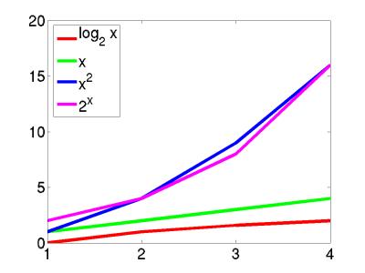
Let's consider the following algorithms on an array whose length is n. (I'm assuming you're familiar with these algorithms; give a yell if not.)
- Returning the first element takes an amount of time that is independent of n ("constant time")
- Binary search runs in time proportional to log(n)
- Sequential search runs in time proportional to n
- Many sorting algorithms (such as selection sort) run in time proportional to n². So does any algorithm that deals with all the pairs of numbers runs in time proportional to n² (think of a round-robin tournament).
For example, given {1, 2, 3, 4, 5}, compute:
There are n rows and n columns, so n*n entries.1+1 2+1 ... 5+1 1+2 2+2 ... 5+2 1+3 2+3 ... 5+3 1+4 2+4 ... 5+4 1+5 2+5 ... 5+5 - Algorithms that deal with all possible combinations of the items
run in time 2n.
For example, given {1, 2, 3, 4, 5}, compute:- 1, 2, 3, 4, 5
- 1+2, 1+3, 1+4, 1+5, 2+3, 2+4, 2+5, 3+4, 3+5, 4+5
- 1+2+3, 1+2+4, 1+2+5, 1+3+4, 1+3+5, ...
- 1+2+3+4, ...
- 1+2+3+4+5, ...
Now, computers are always getting faster, but these "orders of growth" help us see at a glance the inherent differences in run-time for different algorithms.
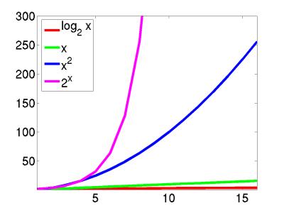
Clearly, when designing algorithms we need to be careful. For example, a brute-force chess algorithm has runtime 2n which makes it completely impractical. Interestingly, though, this type of complexity can help us. In particular, the reason that it is difficult for someone to crack your password is because the best known algorithm for cracking passwords runs in 2n time (specifically factoring large numbers into primes).
Asymptotic notation
So if we're willing to characterize an overall "order of growth", as above, we can get a handle on the major differences. This notion of "grows like" is the essence of the running time — linear search's running time "grows like" n and binary search's running time "grows like" log(n). Computer scientists use it so frequently that we have a special notation for it: "big-Oh" notation, which we write as "O-notation."
For example, the running time of linear search is always at most some linear function of the input size n. Ignoring the coefficients and low-order terms, we write that the running time of linear search is O(n). You can read the O-notation as "order." In other words, O(n) is read as "order n." You'll also hear it spoken as "big-Oh of n" or even just "Oh of n."
Similarly, the running time of binary search is always at most some logarithmic function of the input size n. Again ignoring the coefficients and low-order terms, we write that the running time of binary search is O(lg n), which we would say as "order log n," "big-Oh of log n," or "Oh of log n."
In fact, within our O-notation, if the base of a logarithm is a constant (like 2), then it doesn't really matter. That's because of the formula
loga n = (logb n) / (logb a)for all positive real numbers a, b, and c. In other words, if we compare loga n and logb n, they differ by a factor of logb a, and this factor is a constant if a and b are constants. Therefore, even though we use the "lg" notation within O-notation, it's irrelevant that we're really using base-2 logarithms.
O-notation is used for what we call "asymptotic upper bounds." By "asymptotic" we mean "as the argument (n) gets large." By "upper bound" we mean that O-notation gives us a bound from above on how high the rate of growth is.
Here's the technical definition of O-notation, which will underscore both the "asymptotic" and "upper-bound" notions:
A running time is O(n) if there exist positive constants n0 and c such that for all problem sizes n ≥ n0, the running time for a problem of size n is at most cn.
Here's a helpful picture:
The "asymptotic" part comes from our requirement that we care only about what happens at or to the right of n0, i.e., when n is large. The "upper bound" part comes from the running time being at most cn. The running time can be less than cn, and it can even be a lot less. What we require is that there exists some constant c such that for sufficiently large n, the running time is bounded from above by cn.
For an arbitrary function f(n), which is not necessarily linear, we extend our technical definition:
A running time is O(f(n)) if there exist positive constants n0 and c such that for all problem sizes n ≥ n0, the running time for a problem of size n is at most c f(n).
A picture:
Now we require that there exist some constant c such that for sufficiently large n, the running time is bounded from above by c f(n).
Actually, O-notation applies to functions, not just to running times. But since our running times will be expressed as functions of the input size n, we can express running times using O-notation.
In general, we want as slow a rate of growth as possible, since if the running time grows slowly, that means that the algorithm is relatively fast for larger problem sizes.
We usually focus on the worst case running time, for several reasons:
- The worst case time gives us an upper bound on the time required for any input.
- It gives a guarantee that the algorithm never takes any longer.
- We don't need to make an educated guess and hope that the running time never gets much worse.
You might think that it would make sense to focus on the "average case" rather than the worst case, which is exceptional. And sometimes we do focus on the average case. But often it makes little sense. First, you have to determine just what is the average case for the problem at hand. Suppose we're searching. In some situations, you find what you're looking for early. For example, a video database will put the titles most often viewed where a search will find them quickly. In some situations, you find what you're looking for on average halfway through all the data…for example, a linear search with all search values equally likely. In some situations, you usually don't find what you're looking for.
It is also often true that the average case is about as bad as the worst case. Because the worst case is usually easier to identify than the average case, we focus on the worst case.
Computer scientists use notations analogous to O-notation for "asymptotic lower bounds" (i.e., the running time grows at least this fast) and "asymptotically tight bounds" (i.e., the running time is within a constant factor of some function). We use Ω-notation (that's the Greek leter "omega") to say that the function grows "at least this fast". It is almost the same as Big-O notation, except that is has an "at least" instead of an "at most":
A running time is Ω(n) if there exist positive constants n0 and c such that for all problem sizes n ≥ n0, the running time for a problem of size n is at least cn.
We use Θ-notation (that's the Greek letter "theta") for asymptotically tight bounds:
A running time is Θ(f(n)) if there exist positive constants n0, c1, and c2 such that for all problem sizes n ≥ n0, the running time for a problem of size n is at least c1 f(n) and at most c2 f(n).
Pictorially,
In other words, with Θ-notation, for sufficiently large problem sizes, we have nailed the running time to within a constant factor. As with O-notation, we can ignore low-order terms and constant coefficients in Θ-notation.
Note that Θ-notation subsumes O-notation in that
If a running time is Θ(f(n)), then it is also O(f(n)).
The converse (O(f(n)) implies Θ(f(n))) does not necessarily hold.
The general term that we use for either O-notation or Θ-notation is asymptotic notation.
Recap
Both asymptotic notations—O-notation and Θ-notation—provide ways to characterize the rate of growth of a function f(n). For our purposes, the function f(n) describes the running time of an algorithm, but it really could be any old function. Asymptotic notation describes what happens as n gets large; we don't care about small values of n. We use O-notation to bound the rate of growth from above to within a constant factor, and we use Θ-notation to bound the rate of growth to within constant factors from both above and below.
We need to understand when we can apply each asymptotic notation. For example, in the worst case, linear search runs in time proportional to the input size n; we can say that linear search's worst-case running time is Θ(n). It would also be correct, but less precise, to say that linear search's worst-case running time is O(n). Because in the best case, linear search finds what it's looking for in the first array position it checks, we cannot say that linear search's running time is Θ(n) in all cases. But we can say that linear search's running time is O(n) in all cases, since it never takes longer than some constant times the input size n.
Working with asymptotic notation
Although the definitions of O-notation and Θ-notation may seem a bit daunting, these notations actually make our lives easier in practice. There are two ways in which they simplify our lives:
- Constant factors don't matter
- Constant multiplicative factors are "absorbed" by the multiplicative constants in O-notation (c) and Θ-notation (c1 and c2). For example, the function 1000n2 is Θ(n2), since we can choose both c1 and c2 to be 1000. Although we may care about constant multiplicative factors in practice, we focus on the rate of growth when we analyze algorithms, and the constant factors don't matter. Asymptotic notation is a great way to suppress constant factors.
- Low-order terms don't matter
- When we add or subtract low-order terms, they disappear when using asymptotic notation. For example, consider the function n2 + 1000n. I claim that this function is Θ(n2). Clearly, if I choose c1 = 1, then I have n2 + 1000n ≥ c1n2, so this side of the inequality is taken care of.
The other side is a bit tougher. I need to find a constant c2 such that for sufficiently large n, I'll get that n2 + 1000n ≤ c2n2. Subtracting n2 from both sides gives 1000n ≤ c2n2 – n2 = (c2 – 1) n2. Dividing both sides by (c2 – 1) n gives 1000 / (c2 – 1) ≤ n. Now I have some flexibility, which I'll use as follows. I pick c2 = 2, so that the inequality becomes 1000 / (2 – 1) ≤ n, or 1000 ≤ n. Now I'm in good shape, because I have shown that if I choose n0 = 1000 and c2 = 2, then for all n ≥ n0, I have 1000 ≤ n, which we saw is equivalent to n2 + 1000n ≤ c2n2.
The point of this example is to show that adding or subtracting low-order terms just changes the n0 that we use. In our practical use of asymptotic notation, we can just drop low-order terms.
In combination, constant factors and low-order terms don't matter. If we see a function like 1000n2 – 200n, we can ignore the low-order term 200n and the constant factor 1000, and therefore we can say that 1000n2 – 200n is Θ(n2).
As we have seen, we use O-notation for asymptotic upper bounds and Θ-notation for asymptotically tight bounds. Θ-notation is more precise than O-notation. Therefore, we prefer to use Θ-notation whenever it's appropriate to do so. We shall see times, however, in which we cannot say that a running time is tight to within a constant factor both above and below. Sometimes, we can only bound a running time from above. In other words, we might only be able to say that the running time is no worse than a certain function of n, but it might be better. In such cases, we'll have to use O-notation, which is perfect for such situations.
List analysis
Both list implementations support the same interface. When would we choose one over the other?
Linked list: efficient if we're adding / removing / getting / setting at the front of the list. Constant time, in fact. But in the worst case we might have to advance all the way through the list — Θ(n).
Growing array: efficient if we're getting / setting an index already within the size of the filled in elements. Adding / removing at the end is efficient (except when we have to grow), but in the worst case we might have to shift over the entire array — Θ(n). What about that growing bit? While any individual growing step will be slow, it doubles the length of the array, so will last a while. Thus we won't have to grow it again till we add as many elements to the array as we already have. Thus on average, it's not so expensive.
We can make this argument tighter, and argue that n add operations will never take more than O(n) time. This is O(1) amortized time. Amortization is what accountants do when saving up to buy an expensive item like a computer. Suppose that you want to buy a computer every 3 years and it costs $1500. One way to think about this is to have no cost the first two years and $1500 the third year. An alternative is to set aside $500 each year. In the third year you can take the accumulated $1500 and spend it on the computer. So the computer costs $500 a year, amortized. (In tax law it goes the other direction - you spend the $1500, but instead of being able to deduct the whole thing the first year you have to spead it over the 3 year life of the computer, and you deduct $500 a year.)
For the growing array case, we can think in terms of tokens that can pay for copying an element. We charge 3 tokens for each add. One pays for adding the item to the array and two are set aside for later. Suppose that we have just expanded the array from size n to size 2n and copied the items in the old array to the first n positions of the new array. We have no accumulated tokens. The last n positions of the array are empty, so we will be able to do n add operations before the new array is full with 2n items in it. Each add sets aside 2 tokens. After n add operations we will have accumulated 2n tokens. That is enough to pay for copying all 2n things in the array when we do the next add and have to double the array size again. Therefore the cost is O(1) per add operation, amortized. (The current implementation of ArrayList in Java makes the new array 3/2 times the size of the old array to waste less space, but the argument can be modified to show that a charge of 4 tokens works.)
Iteration
Our list interface is sufficient to do lots of things with lists. For example, we can see if an element appears in the list by getting each item and seeing if it's what we wanted, and we can test equality of two lists by marching down each of them in tandem and comparing items.
This style of going through a data structure is so common that there's a name for it: an iterator. Java supports iteration with a standard Iterator interface, which abstracts the pattern of looping over every item in a container. In fact, it's the basis for the for-each loop that we've been using:
for (Blob b : blobs) {
  b.step();
}
Contrast this with what we'd have to write with a traditional indexed for-loop:
for (int i=0; i<blobs.size(); i++) {
  blobs.get(i).step();
}
There are several advantages to the for-each loop. It's just easier to read, once you're used to it (which hopefully you are by now, if you weren't before!). The indexed for-loop has a variable i that serves no purpose other than to step through the items — we don't actually care what its value is, so it's in some sense extraneous. And one should never waste bits! Perhaps most importantly in this example, the indexed for-loop is much less efficient for a linked-list implementation. Recall that the way get works in a linked list is that it starts at the beginning, and steps down the list the specified number of times. So each time through the loop, we go back to the start of the list again, rather than just picking up where we left off. This actually leads to a quadratic algorithm! For each i, we have to advance i times from the start. And 1+2+3+...+n is n*(n+1)/2, which is O(n^2).
An iterator keeps track of where it is in the iteration, so can be more efficient. At its heart, an iterator has two methods: hasNext tells us whether or not there's something left to get, and next gets it and advances the iteration. So our for-each loop is really:
for (SimpleIterator<Blob> i = blobs.newIterator(); i.hasNext(); ) {
  i.next().step();
}
Note that the "advance" part of the for loop is empty, as the next call in the body of the loop both gets the next thing and advances so that a subsequent call will be for the subsequent element. That is:
SimpleIterator<Blob> i = blobs.newIterator();
Blob b0 = i.next(); // return the 0th element [if there is one; else exception]
Blob b1 = i.next(); // returns the 1st element [if there is one; else exception]
Now, the iterator-based loop is no more (and perhaps) less readable than the int-counter loop. But it (might be) more efficient, as the iterator can "remember" where it is, and not have to go back to the beginning each time. And with a bit of "syntactic sugar", we can write a beautiful for-each loop and rely on our language to compile it down into an iterator, without us even having to think about that. The iterator version also makes clear exactly what the loop is all about.
Now details. Look at the interface for the iterator, SimpleIterator.java, and an expanded interface for list including it SimpleIList.java. Then a full example of the indexed and iterator loops in action: IterTest.java.
The implementation of an iterator for a linked list just keeps a pointer to an element, and advances by the next when asked to. When we reach the end (null), we indicate that there is no next. ISinglyLinked.java.
For a growing array, we keep the current index into the array, incrementing by 1 each time, until we reach the size of the array. IGrowingArray.java. (Note that there's no performance issue here either way, as the array is random access.)
The Java list iterator, as well as that described in the book, is quite a bit fancier. It supports moving bidirectionally (in a doubly linked implementation), adding/removing/replacing at the current position, etc. But the basic idea of packaging up a position into a list remains the same.