Since we basically use the Bag-of-Words features for all our classifiers, the feature dimension is
immediately defined by the vocabulary size of the data set. Having an original feature
dimension of more than 60000, we not only risk including large amount of noises in our
classifiers, but also suffer from technical problems such as memory and speed issues.
Thus we have to first explore possible ways of reducing the dimensionality of the data
set.
We initially considered applying PCA to our data set. However, PCA will project the data set
onto a completely new set of bases, thus rendering all the features meaningless as opposed to the
Bag-of-Words features we intended. So our dimensionality reduction will be carried out via
feature selections.
We explore two different feature selection metrics: Impurity Measures, and Posterior Variances, as discussed below.
One metric that we use is Impurity Measures, inspired by the test selection method of the decision tree construction procedure. For each binary feature s, we define its impurity measure to be
where

and
The lower the impurity measure is, the better the feature is.
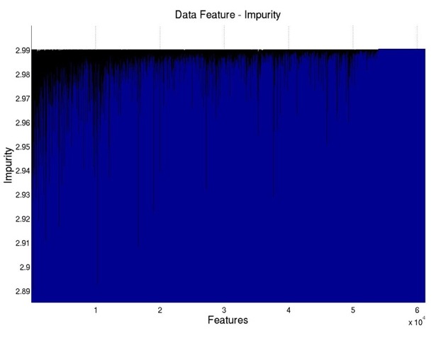
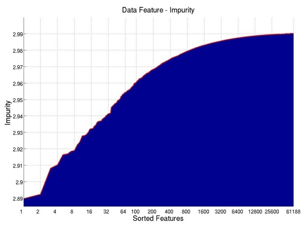
As shown in Figure 1, the plot on the left shows the impurity measures for all the features. If
we sort all the features according to their impurity measures, we get the plot on the
right. It can be seen that after the first 3200 features (about 5.2% of all the features),
the impurity measure already grows really slow, indicating possible ways of selecting
features.
Another metric that we use is Posterior Variances. For each feature s, we carry out the following
calculation: we, for all class labels y  Y , calculate all the posterior probabilities Pr(y|s = 1), we
then calculate the variance of this set of posteriors. The higher the variance is, the better the
feature is.
Y , calculate all the posterior probabilities Pr(y|s = 1), we
then calculate the variance of this set of posteriors. The higher the variance is, the better the
feature is.
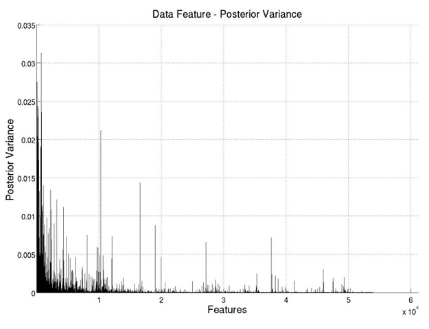
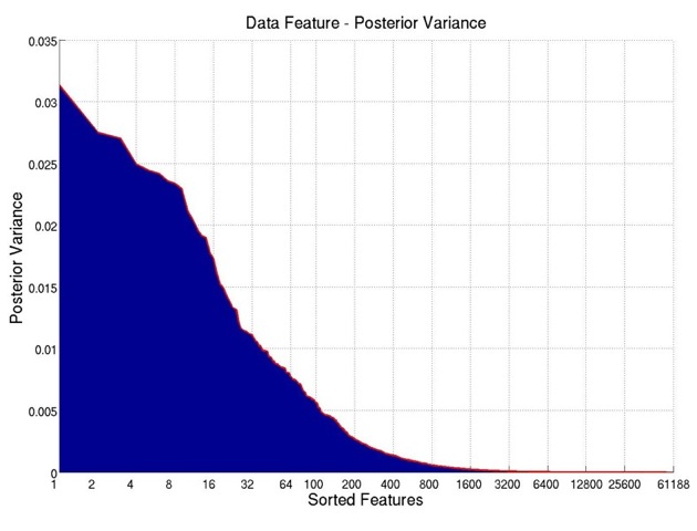
As shown in Figure 2, the plot on the left shows the posterior variances for all the
features. If we sort all the features according to their posterior variances, we get the plot
on the right. It can be seen that after the first 1600 features (about 2.6% of all the
features), the posterior variance is already really low, indicating possible ways of selecting
features.