3 Classifiers and Combination Strategies

In this section, we discuss all the classifiers, as well as the multiple strategies of combining them, that we use in the classification task.

3.1 Single Classifiers

The basic single classifiers that we use are Naïve Bayes, kNN, and Multi-SVM. We omit detailed introduction of these classifiers since they are covered in our lectures as well as in the text [1].

Each of the three actually corresponds to a set of classifiers in our experiments, since we have different metrics and can select features of different dimensions. More specifically, we experiment with both of our feature selection metrics: Impurity Measures and Posterior Variances, and of nine different feature dimensions: {100,200,400,800,…,25600}.

Next we show the results of separately applying each of these three sets of classifiers on the 20Newsgroups data set.

3.1.1 Naïve Bayes

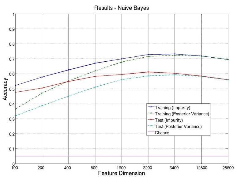
Figure 3 shows the training and test accuracies of the set of Naïve Bayes classifiers.

Figure 3: Training and Test Accuracies of Naïve Bayes

As can be seen, for both of the feature selection metrics, the highest training and test accuracies are achieved at the feature dimension of around 3200 and 6400. The highest test accuracy is around 61.1% and appears at the feature dimension of 3200. It is more than 10% higher than applying Naïve Bayes on the original data set, and is only using about 5.2% of all the original features.

3.1.2 kNN

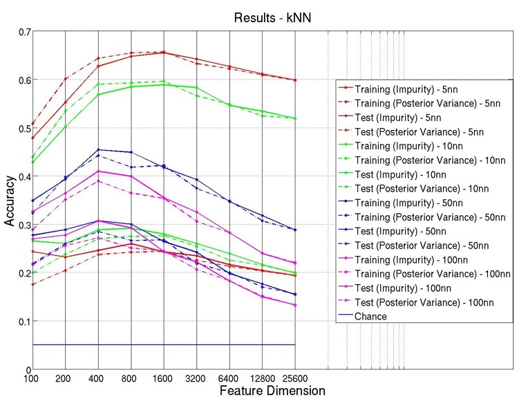
Figure 4 shows the training and test accuracies of the set of kNN classifiers. Note that not only do these set of classifiers differ in the feature selection metrics and dimensions, we also experiment on kNN with different values of the number of neighbors: k {5,10,50,100}.

Figure 4: Training and Test Accuracies of kNN

As shown, there are roughly three clusters of curves, where the bottom cluster corresponds to the test accuracies. Most of the test accuracies are below 30%, which are better than chance (5%), but are still quite low compared to other sets of classifiers. This trend also agrees to that of our preliminary results, suggesting that kNN might just not be a good choice for our information classification task.

3.1.3 Multi-Class SVM

We use the one-versus-one strategy to implement the multi-class SVM. Namely for K labels, we train different binary SVMs (one for each pair of classes). Then for each test example we assign its label according to the majority vote among all the binary classifiers. And for each binary SVM, we use Sequential Minimal Optimization method to find the separating hyperplane.

In our implementation, we use Matlab’s svmsmoset function to set the optimization options, the svmtrain function to train the model and svmclassify functions to infer the label.

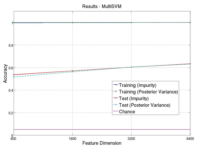
When experimenting on low-dimensional data (d {100,200,400}), trainings failed to converge due to lack of enough features, and when on high-dimensional data (d {12800,25600}), we encounter out of memory problems. Therefore, our results only include the ones from experiments on data of dimensions d {800,1600,3200,6400}.

Figure 5: Training and Test Accuracies of Multi-SVM

Figure 5 shows the training and test accuracies of our experiments. It can be seen that the training accuracy is almost 100% for all feature selection metrics and dimensions, and the test accuracy gradually increases as feature dimension increases.

3.2 Classifier Combinations

We experiment with the following set of classifier combination approaches.

• Random selection - We train every single classifier on the training data. Then for each test document, we randomly select a classifier to label it.
• Majority Vote - We train every single classifier on the training data. Then for each test document, we assign its label according to the majority vote of all the classifiers.
• Highest Confidence Vote - We train every single classifier on the training data. Then for each test document, we assign its label according to label produced by the classifier with the highest confidence (We have each of the single classifiers outputting a naïve confidence, and then map all the confidence measures to the interval [0,1] as a way of normalization, to make them comparable).
• Dynamic Classifier Selection [2] - We train every single classifier on the training data. For each test document, we first select an neighborhood of it from the training data, we then compute the training accuracy of all the classifiers on this neighborhood. The classifier with the highest accuracy is then used to label the test document.

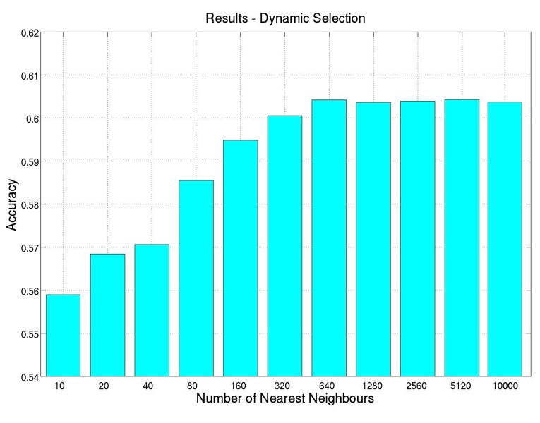
The first three combination strategies are rather straightforward and contain little variability. For Dynamic Classifier Selection, the key point is how to, for a test example, choose its neighborhood among the training examples, since we will select a classifier to use depending on the accuracies of all the classifiers on this neighborhood.

In our experiment, we, for each test example, select K-nearest data points from the training set as its neighborhood (We tried carrying out the distance calculation on the original training data, as well as on the different dimension-reduced training data corresponding to the specific feature selection metric and dimension of each of the single classifiers. It turned out that the former method worked better). We experiment with different K’s, in order to find a K that produces the best result.

Figure 6: Test Accuracies of Dynamic Selection of Different Neighbour Sizes

The results of these experiments are shown in Figure 6. We can see that, initially the accuracy increases as the neighborhood enlarges, however, after the size reaches and goes beyond 640, the accuracy stops increasing and remains relatively unchanged. Thus, we are picking K = 640 for our dynamic selection combination strategy.

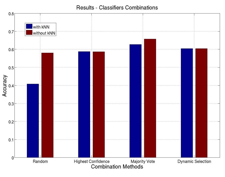
As previously discussed, the accuracies of all the kNN classifiers are quite low. So we carry out two sets of combination experiments; one with kNN classifiers and the other without. The results are shown in Figure 7.

Figure 7: Test Accuracies of Different Combination Strategies with/without kNN

As can be seen, excluding the kNN classifiers actually produces better results than including them: it has no effects on highest confidence and dynamic selection methods, but brings improved accuracies on random selection and majority vote methods. Therefore, we exclude the set of kNN classifiers from the combination methods.